Finite Impulse Response Filter

The Finite Impulse Response (FIR) filter is a classic system. Without going into hyperbolics, it is hard to overemphasize how important and versatile it is...I mean it is essentially performing convolution for us. As I said in lecture, it can be used for tons of things.

The math formula for it is pretty easy...the output at any point in time is the sum of a certain number of past values (A finite number of them), each multiplied by the appropriate coefficients. This can readily be envisioned in a digital system:

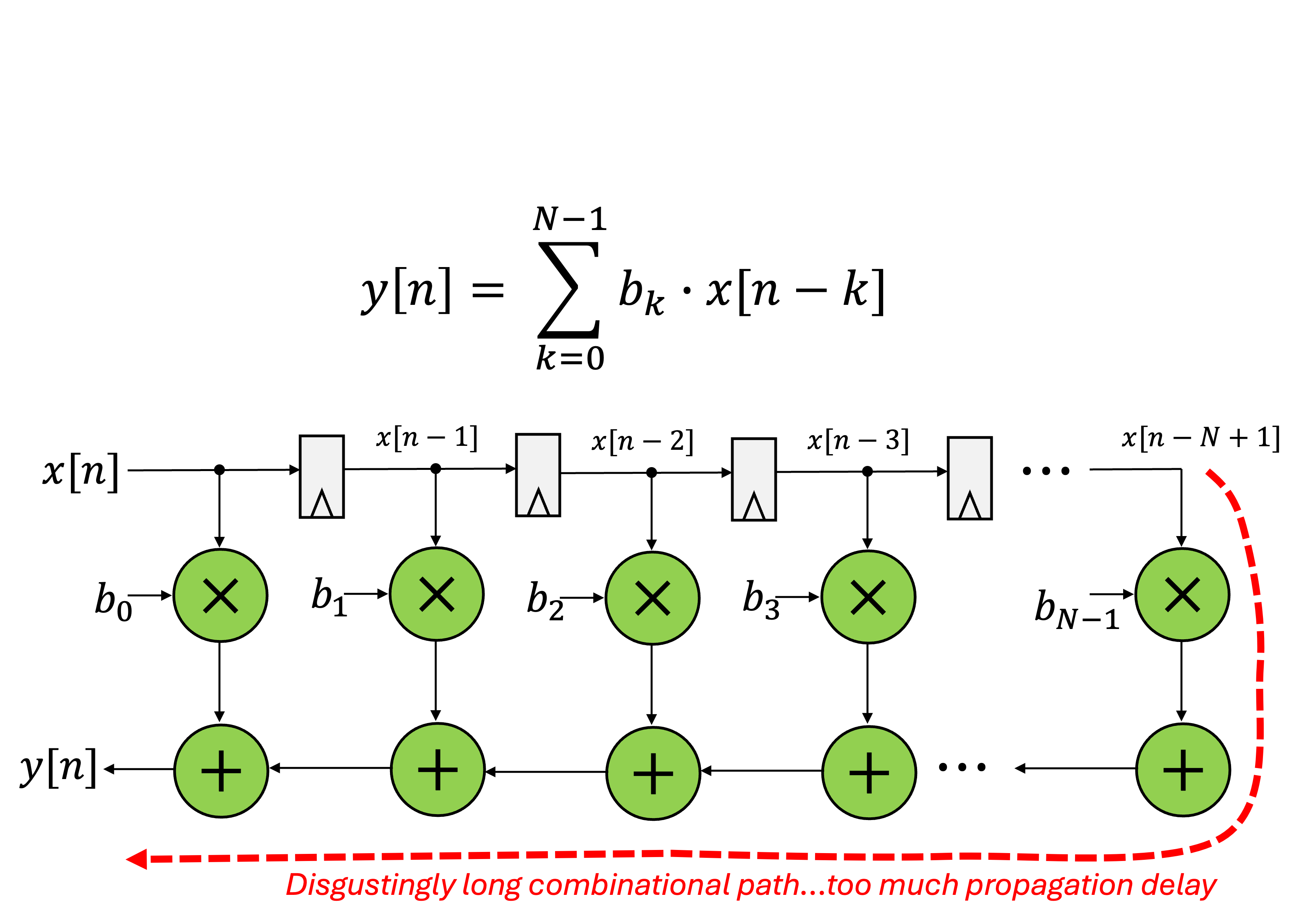
That design has a lot of timing issues, in particular a potentially awful critical path. Refactoring the timing can yield an equivalent design that looks like the following:

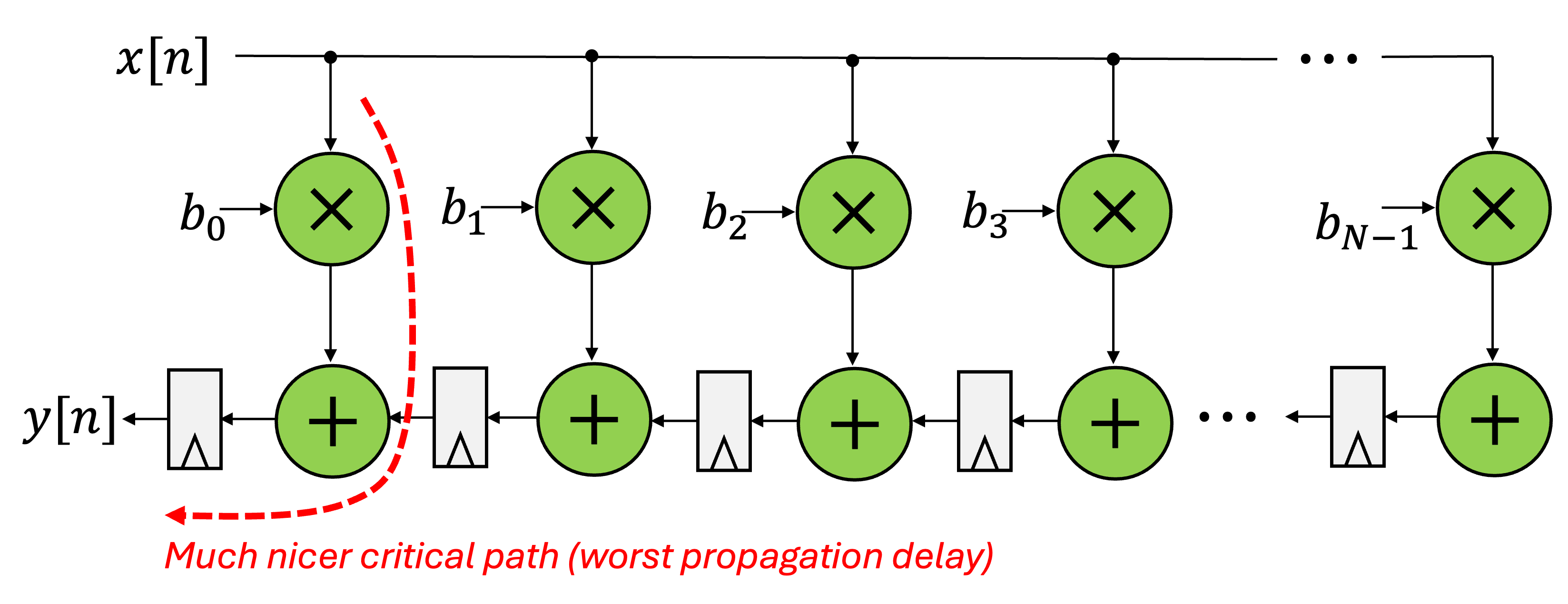
This is what we'll try to design this week. Think about how this would look in Verilog....think about how it could be made extensible/parameterizable. Probably some for loops, yeah?

Our FIR Design

There's many ways to write a FIR filter. We're going to make a simple 15-tap FIR filter for today (and then later on if you want to expand it or parameterize it), great, but 15 is good enough for now.

The starting skeleton is below:

module fir_15
	(
        input wire clk,
        input wire rst,
        input wire signed [31:0] data_in,
        input wire data_in_valid,
        input wire signed [NUM_COEFFS-1:0][7:0] coeffs,
        output logic signed [31:0] data_out,
        output logic data_out_valid
	);
    localparam NUM_COEFFS = 15;
    //your design here.
endmodule

The ports are as follows:

• clk: Your clock signal
• rst: Your reset signal
• [31:0] data_in: This is your input signal. This is a signed value.
• data_in_valid: Signal indicating when data_in has new data.
• [NUM_COEFFS-1:0][7:0] coeffs: For this lab, this is a fifteen-long array of 8 bit signed coefficients for our FIR taps. For a few reasons relating to Vivado, we have to keep this as a double-packed array and cannot use unpacked dimensions. These coefficients will be changeable "in real time" when we dump this onto the FPGA so we can't have the coefficients as constants or parameters or something.
• [31:0] data_out: Output signal.
• data_out_valid: Signal indicating when data_out has new data.

Build the FIR based on the rough "schematic" above. There should be one cycle of latency between when data comes in and when it comes out (there does not need to be a build-up phase that you'll sometimes see with convolutional filters when enough data hasn't been inputted yet). For right now you do not need to worry about bit-growth in our signals. You can assume that we'll be putting in relatively small signals to the input (likely 8 bits and therefore we'll likely only be ending up with ~20 bits of precision we need to worry about).

You should not assume that good data_in is necessarily coming in every clock cycle. data_in_valid dictates when "good" data is on the input. If there is no valid data on a clock cycle, the FIR should not "evolve." This will be important when we start integrating it into frameworks where samples are not coming in at every clock cycle. For examples, if your FIR is running at 100 MHz, but you're dealing with data that is coming in at 25 Msps, you would expect, on average, one data_in_valid every four clock cycles, and you should be generating one data_out_valid every four clock cycles as well.

Testing

Now how could we test such a signal-processy type system? You could look at waveforms, or you could even write a Python implementation of a FIR, like we've already done, but why waste the time. One of the great things about Python is have you have access to many "gold-standard" type implementations of things, and FIR filters are one of them. Yes, Scipy is a Python library, but it is actually really just a light Python wrapper surrounding a golden core of highly optimized C.

If you go ahead and import scipy (or pip install if you don't have it already), you can quickly get access to a FIR filter.

A few lines like this:

from scipy.signal import lfilter

and this (assuming you have FIR coefficients as coeffs and the signal as samples):

model_output = lfilter(coeffs, [1.0], samples)

Is enough to give you access to a true, good software FIR implementation that we can compare our HDL against. I think this is one of the key strengths of using a language like Python for verification.

Signals

Now what should we put in? Well likely some signals to test. An easy thing to do would be a few sine waves of different amplitudes.

To help get you started I made this fancy little function that can take in a list of frequencies and amplitudes and as well as sample rate and duration and gives you a full signal.

def generate_signed_8bit_sine_waves(sample_rate, duration,frequencies, amplitudes):
    """
    frequencies (float): The frequency of the sine waves in Hz.
    relative amplitudes (float) of the sinewaves (0 to 1.0).
    sample_rate (int): The number of samples per second.
    duration (float): The duration of the time series in seconds.
    """
    num_samples = int(sample_rate * duration)
    time_points = np.arange(num_samples) / sample_rate
    # Generate a sine wave with amplitude 1.0
    result = np.zeros(num_samples, dtype=int)
    assert len(frequencies) == len(amplitudes), "frequencies must match amplitudes"
    for i in range(len(frequencies)):
        sine_wave = amplitudes[i]*np.sin(2 * np.pi * frequencies[i] * time_points)
        # Scale the sine wave to the 8-bit signed range [-128, 127]
        scaled_wave = sine_wave * 127
        # make 8bit signed integers:
        result+=scaled_wave.astype(np.int8)
    return (time_points,result)

#time and signal input:
t,si = generate_signed_8bit_sine_waves(
    sample_rate=100e6,
    duration=10e-6,
    frequencies=[46e6,20e6, 200e3],
    amplitudes=[0.1,0.1, 0.5]
)

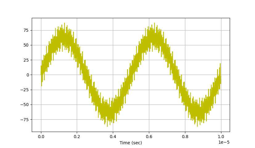
Just running matplotlib's plotter on the above signal gives you this, which is what we expect. Two sine waves of relatively small amplitude but large frequency (46MHz and 20 MHz) and then one of larger amplitude but lower frequency (200 kHz).

With this and scipy and cocotb and matplotlib and your intelligence you should be able to compare your HDL FIR module to the software model. That is your goal!

An Annoyance

One annoying thing that we have to deal with is the two packed dimensions of [NUM_COEFFS-1:0][7:0] coeffs. Ideally, we'd actually have specified this input with one packed and one unpacked dimension like so: [7:0] coeffs [NUM_COEFFS-1:0] since that is a more natural way to think about it, but Vivado's Verilog and block diagram environment does not play well with those so we need to stick with only packed dimensions. You'll see when you run waveforms (or when you're into Vivado later) that this array is just going to get handed around like a [119:0] long thing. This isn't wrong, since multiple packed dimensions are basically just sub-indexing shorthand (just like multidimensional arrays in C), but Cocotb uses them like this as well too. The upcoming (or already happened) 2.0 release will fix this a bit with its logic slices, but we're stuck in 1.9.2 for right now. A cheap way to put all the bits into this full 2D array is like so:

    for i in range(15):
        for b in range(8):
            dut.coeffs[b+8*i].value = (coeffs[i]>>b)&0x1

You might find that useful for your testbenching.

Coefficients

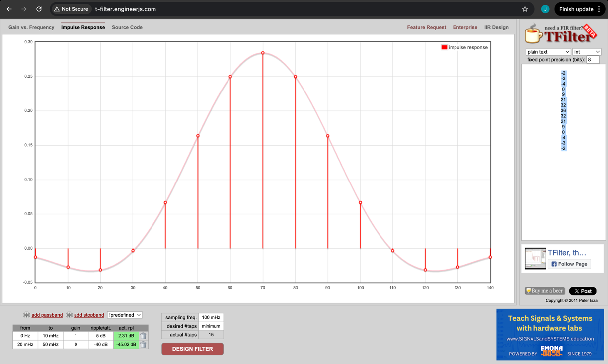
We're designing an FIR filter. We have 15 taps and for the sake of our testing let's restrict the taps to 8 bits in size for now. That's still 1.33\times10^{36} possible tap combinations so there's a lot of design space. We could try each one out one at a time, but there are better ways. Matlab, Scipy, Numpy all have some cool FIR design tools you can try if you like. There is a classic (internet class) tool to design these on the web found here. You can basically tell it the pass bands and stop bands and various levels you want to pass/block at. We'll aim for a pass band out to 10 MHz with the stop band existing from 20 MHz up (at a 100 MHz sample rate). Entering those specs in will give us the following coefficients:

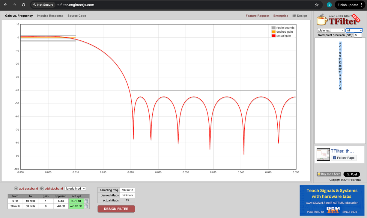
You can also, on that site, see what the impulse response would be too (this may be helpful...especially when looking at signals on the monitor later).

I chose to use the coefficients in their 8-bit integer form since that is the easiest for us to deploy (avoid floats unless you really need them).

Getting Results

Now with all these parts in place, write a testbench that drives in a set set of signals (perhaps the one we show you how to generate above, though feel free to pick other signals if you'd like, provided they are non-trivial).

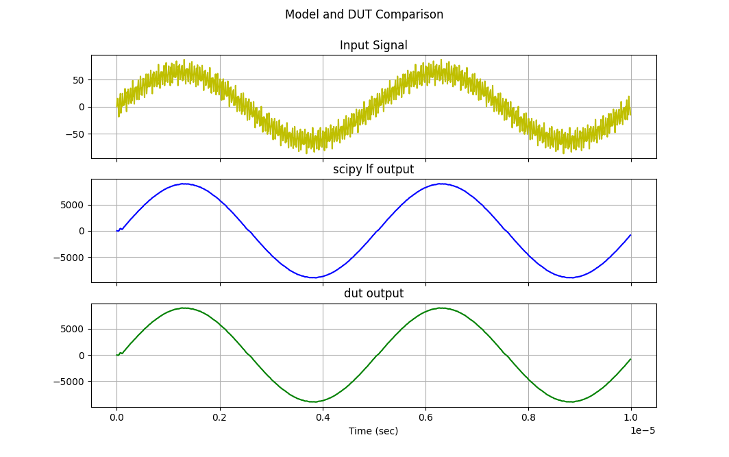
Run the signal through both the Scipy Reference model and your Verilog DUT. Plot them side-by-side-by-side to see if they match up or not!

Here's my result using these coefficients: [-2,-3,-4,0,9,21,32,36,32,21,9,0,-4,-3,-2] which is a low-pass filter (the same one shown above).

And here's my result using these (different) coefficients: [-3,14,-20,6,16,-5,-41,68,-41,-5,16,6,-20,14,-3] which is a high-pass filter.

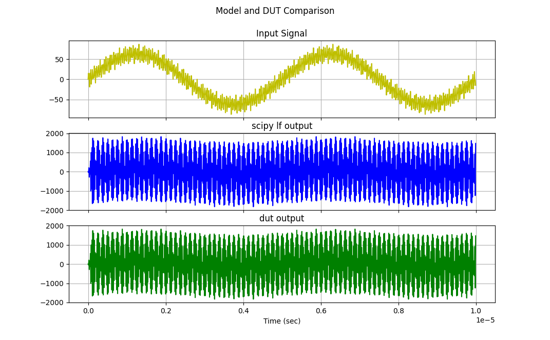
You should be generating something similar.

One thing you'll likely note is that the sheer magnitude of the output signals will often be much larger than the input signal. This is a byproduct of us only using integers as our terms. It is related to the concept of bit-growth, but isn't exactly the same concept. Ideally we'd be using FIR tap coefficients that have the same relative weights to one anther, but which all sum to a total weighting of about unity. But we only have integers to play with (8 bit ones) and since our incoming signals are also only integers the signal can grow.

A easy fix for this is to allow the numbers to grow in size and then when you get to the end, divide the result by the sum of all the coefficients. We'll do somethign similar to that in the next part of this week's assignments and is good enough for today. If you have a much larger FIR, delaying dealing of value growth and bit-growth until the completion of the summations can be problematic and there are certain ways to deal with it. For now don't worry about it.

When complete, upload your working FIR filter and your testbench below. I should be able to download both and test them and get a sweet looking plot (similar to above), but maybe with some different signals and coefficients.

Upload your final "verified" fir15.sv here!

Select File No file selected

Ask for Help Loading...

Upload your testbench here!

Select File No file selected

Ask for Help Loading...