RFSoC

The Next Board

The questions below are due on Friday October 24, 2025; 11:59:00 PM.

You are not logged in.
Please Log In for full access to the web site.
Note that this link will take you to an external site (https://shimmer.mit.edu) to authenticate, and then you will be redirected back to this page.

The Setup

OK this should literally start exactly where you left off in week 6 with the RFSoC. We're going to do a few things:

Reclock the datapath. Instead of the nasty 147.XYZ MHz of last week, we're going to play some games with the DDC and clock to get everything to 64 MHz. This should make things much easier to work with later on.
Decimate down to 250 ksps (rather than 64 Msps). As we talked about earlier this term, to do this, we need to run an anti-aliasing filter on both signals and then take 1/256 samples. We'll use a piece of IP to do this for us.
Possibly update the iq_framer you wrote last week to now deal with the fact that our decimated sigal pipeline no longer always has data on every clock cycle.
Get the Data into Python and use Python to demodulate, further filter, further downsample, and then finally make a one-second long audio-clip of an FM station that you can play through headphones.

So let's get started.

Sample Rate Adjustment

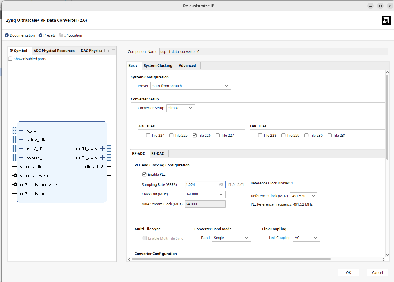
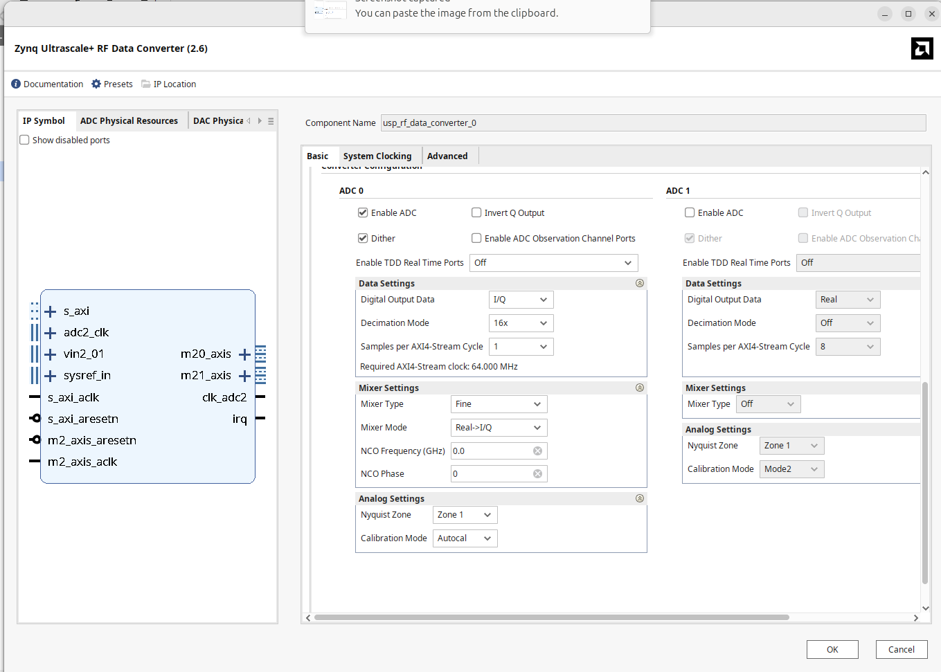
First thing we gotta do is adjust the sample rate of our RFSoC's ADC. Last week it was set to 147.456 MHz because that was a clean derivative signal of the 491.520 MHz clock fed to the RFSoC from the on-board oscillator. This may be a good sample rate for certain applications...for example any signal with a bandwidth of <147.456 MHz could be used with this sample rate in I/Q sampling. But commercial FM is wildly smaller than that (200 kHz). To reconcile this a bit, we're going to adjust our RF Data Converter to sample at 1.024 GHz, decimate by 16 (leading to an outputted sample rate of 64 Msps) and also output a clock at 64 MHz. Doing this means we don't even need a clock wizard anymore to convert between the ADC clock and the sample rate ¹

Update your ADC/Data converter to match the specs described above and listed below. Remember we want 64 Msps I/Q samples one at a time, so one on every clock cycle. There will still be samples always available like last week, just now at a lower sample rate.

Note when you're doing this the data converter IP gui is going to play whack-a-mole with you. You'll change one parameter and then Vivado will change four others in reaction to that, so you will likely need to do several passes on adjusting and setting these different parameters to get everything to work. It is a little annoying, but also kind of expected since all of these options are so interdependent on one another. So be prepared to do double and triple checks.

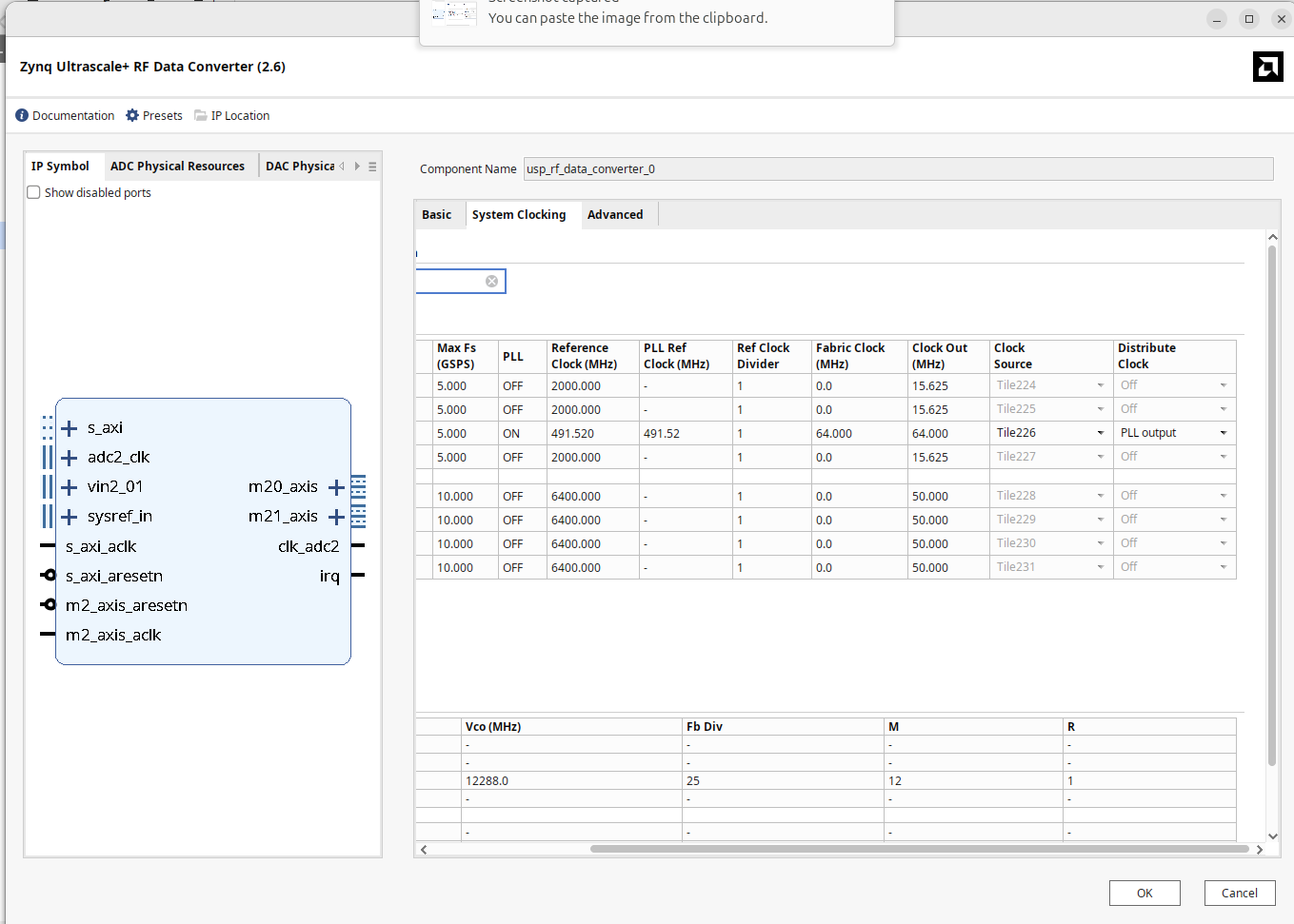
Once done, remove your 11.520 MHz --> 147.456 MHz clock wizard and instead route the 64 MHz clock from the ADC directly to everyhwere the previous 147.456 MHz clock went before.

Optional

If you'd like, feel free to do a build and re-run the Python notebook from last week (updated the sample rate variable to be 64 rather than 147.456 MHz) and you should be getting identical, albeit slightly zoomed-in plots (due to the lower bandwidth).

Filtering and Down-Sampling

Next up we need to actually downsample aggressively even further. Since we are already in a "clean" sample rate of 64 Msps, nice clean 1-in-N decimation factors should also result in relatively clean downsampled sample rates. However!!!! When one down-samples, one must always run the signal through an anti-aliasing (low-pass filter) which is designed to avoid spectral content from different Nyquist zones from folding on top of eachother messing things up. The dataconverter earlier in our pipeline already did this for us before downsampling by a factor of 16 from the original 1.024 Gsps to 64 Msps...now we want to downsample by another factor of 256 to get to a sample rate of 250 ksps.

How should we create our low-pass filter for this? To go from 64 Msps to 250 ksps we'd need to have an LPF with a cutoff at or below 125 kHz. If you go to one of the FIR filter designers and try to do that you'll see a filter with such a super-tiny pass band relative to its large block band will need a lot of taps (hundreds of them). It can be done for sure, but our 15-tap FIR can't do it. We can use the FIR compiler in Vivado so that's another option, but tbh it is an inefficient way of doing what is needed.

The need to downsample and anti-alias filter is ubiquitous in signal processing and instead of using an expensive FIR and then doing the down-sampling in one go, what folks usually do is use a sequence of much simpler low-pass filters which are effectively IIF (Infinite Impulse Response aka recursive filters) and then small baby-step decimation jumps which collectively add up to the ultimate. These types of circuits are known as Cascaded Integrator-Comb Filters. The wikipedia link is good to read through but also this great discussion on CIC filters is also very informative.

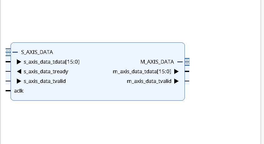
Now we could write one of these, but in the interest of our sanity and time, let's rely on Vivado's built-in CIC compiler core to make one. The datasheet for the CIC Compiler is here. Take a look through it. Using the datasheet and your intuition as a guide, create a CIC which will let us decimate from 64 Msps to 250 ksps (a factor of 256).

Make sure the input and output width are 16 bits. For quantization, use truncation. Also tell the thing to use DSP48 slices (we have several thousand of them, might as well). I believe my CIC uses 9 DSP48 slices (when you look under Implementation). Avoid using TREADY on the output channel. Also use the max number of stages allowable as this will give the best frequency peformance (which you can observe in the Freq Response tab while designing the IP. My filter looked like this when done:

Note this is going to be another whack-a-mole thing...every change you make on one tab will likely change the values you previously set on another so hop back and forth between the tabs to chaperone Vivado as it makes the appropriate design.

You may ask why we should ignore the TREADY output signal. This is totally just a call I made in designing this. You can have TREADY on the output which will then make this CIC support back-pressure. That's fine, but if we just assume that we're always ready to accept data downstream, there's no reason add this in. And also if you do add in the TREADY, you now need to make sure you're asserting it when appropriate so that the filter knows its data is being used and isn't backing itself up.

When done, copy the CIC and make a second identical copy. Insert one CIC module in-between the output of ADC/data converter and each input of your IQ framer module as shown below. Because the CIC filter shouldn't have any non-linear phase or weird things, we can apply one to each of the output channels of the data converter and then feed each of those into the downstream consumer with no issue.

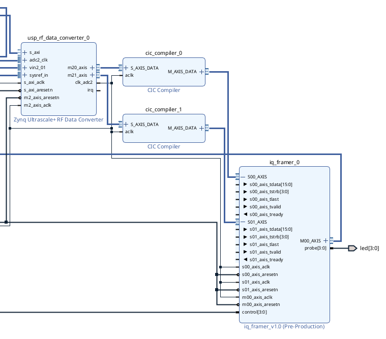
The IQ Framer

Now, depending on how you wrote your IQ framer last week, you may need to update it. Firstly, we want to make sure that we can send up packets of data that are 2^18 in size rather than 2^16. The reason for this is 2^18 will get us a bit above 250,000 and since our sample rate is 250 ksps, that will give us enough samples for one second of audio about. This can be one of several options with switches...I don't care, just make sure you can send up packets of that size. This may not be a thing that matters to you since you already did it.

The second thing your IQ framer may need to get modified to handle is the fact that due to downsampling, there are no longer valid beats of data on every clock cycle. If you designed the CIC filter(s) to have no output TREADY as mentioned, what this means is when data does show up at the output of the CIC (as indicated by Valid), it must be used immediately. We've already been approaching data consumption like that already with the IQ framer. The issue though is that you will not want to be tellign downstream consumers that tvalid is always 1. It would be better to have m00_axis_tvalid be based directly off of s00_axis_tvalid and s01_axis_tvalid. Since both CIC filters should be exactly the same, both tready signals should still be firing together in perfect synchrony, but they will be doing so now once every 256 clock cycles rather than every clock cycle...so make sure the m00_axis_tvalid is based off of the value of at least one of them.

This also therefore means that when running our sample counter, the count (for purposes of TLAST framing) should be incremented ONLY when m00_axis_tvalid && m00_axis_tready are both ready. You may have done this in your design already, but since the samples were always valid from before (because s00_axis_tvalid was always 1) you may have just hard-coded 1's. (I did this originally before modifying it so no shame). Just we're now dealing with and AXI stream where there is not valid data on every frame due to decimation so be aware and double-check your design.

Again if you have issues with this reach out on Piazza or office hours! It shouldn't be too difficult, but I know the whole AXI handshake stuff can get confusing. Happy to send you mine as well.

Putting it All Together

My build ended up looking like this for reference. Notice there's no clock wizard unlike last week.

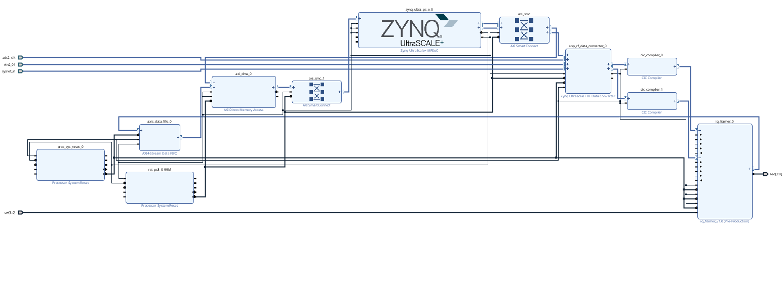
When ready, go ahead and build and everything like before. The generation of output products, in particular for the RF Data Converter takes a decently long time so be prepared.

Again, you need to add a license to your Vivado in order to build. If you're using a machine you haven't used before, you'll have to put the license file on for that machine. Here are the license files for machines 33 to 48 (inclusive) in the lab:

Assuming the build worked out, now it is time to go to Python town.

Python Notebook

Like before, go to the board in the browser, get a new notebook, etc...

from pynq import PL
PL.reset() #important fixes caching issues which have popped up.
import xrfdc #poorly documented library that handles interfacing to the RF data converter
from pynq import Overlay  #import the overlay module
ol = Overlay('./design_1_wrapper.bit')  #locate/point to the bit file
import pprint
pprint.pprint(ol.ip_dict)
dma = ol.axi_dma_0 #might need to change name depending on what you called it
rf = ol.usp_rf_data_converter_0 #might need to change name depending on what you called it
from pynq import Clocks
Clocks.pl_clk0_mhz = 150
print(Clocks.pl_clk0_mhz)

Then let's set our mixer frequency to a station we want to listen to! Pick something, don't just run this code as it is...it will not work!

adc_tile = rf.adc_tiles[2]
print(adc_tile)
adc_block = adc_tile.blocks[0]
print(adc_block)
print(adc_block.BlockStatus)
print(adc_block.MixerSettings)
adc_block.Dither = 0 #doesn't really matter for this lab, but let's turn off.
center_frequency = 1 #Target a radio station you found last week with this (MIT is 88.1... 96.9 is HOT, 100.7 is classic rock, etc...)
adc_block.MixerSettings['Freq']= center_frequency # set the frequency of the Numerically controlled oscillator.
adc_block.UpdateEvent(xrfdc.EVENT_MIXER) #every time setting is changed, must call this.
print(adc_block.MixerSettings)

And finally some stuff that grabs data, chops it up into I and Q and then plots it the spectrum!

import numpy as np
import time
%matplotlib notebook
import matplotlib.pyplot as plt
from pynq import allocate

def plot_to_notebook(time_sec,in_signal,n_samples,):
    plt.figure()
    plt.subplot(1, 1, 1)
    plt.xlabel('Time (usec)')
    plt.grid()
    plt.plot(time_sec[:n_samples]*1e6,in_signal[:n_samples],'y-o',label='Input signal')
    #plt.plot(time_sec[:n_samples]*1e6,in_signal[:n_samples],'y-o',label='Input signal')

    plt.legend()
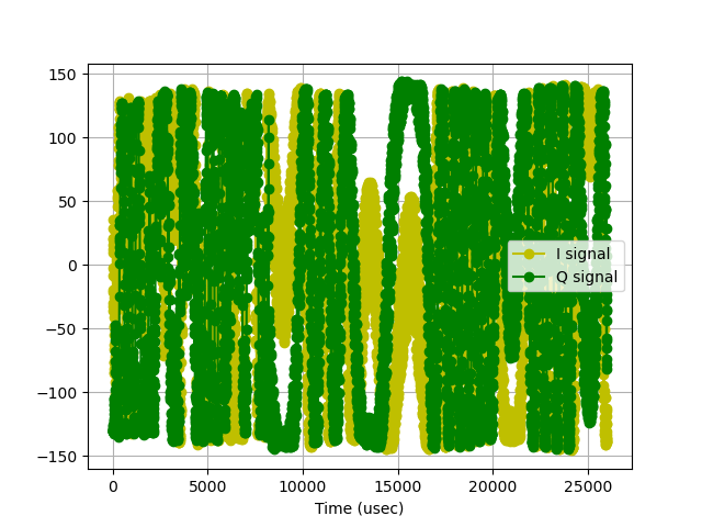
def iq_plot(time_sec,re_signal,im_signal,n_samples,):
    plt.figure()
    plt.subplot(1, 1, 1)
    plt.xlabel('Time (usec)')
    plt.grid()
    plt.plot(time_sec[:n_samples],re_signal[:n_samples],'y-o',label='I signal')
    plt.plot(time_sec[:n_samples],im_signal[:n_samples],'g-o',label='Q signal')
    #plt.plot(time_sec[:n_samples]*1e6,in_signal[:n_samples],'y-o',label='Input signal')

    plt.legend()

def plot_fft(samples,in_signal,n_samples,):
    plt.figure()
    plt.subplot(1, 1, 1)
    plt.xlabel('Frequency')
    plt.grid()
    plt.plot(samples[:n_samples],in_signal[:n_samples],'y-',label='Signal')
    #plt.plot(time_sec[:n_samples]*1e6,in_signal[:n_samples],'y-',label='Signal')
    plt.legend()
# Sampling frequency
fs = 0.25 #new for this week (250 ksps)
# Number of samples
n = 262134 #new for this week (maybe)
T = n/fs
down_from_center =  - fs/2
up_from_center =  + fs/2
# Time vector in seconds
t = np.linspace(0, T, n, endpoint=False)
# Allocate buffers for the input and output signals
ns = np.linspace(down_from_center, up_from_center,n,endpoint=False)
out_buffer = allocate(400024, dtype=np.int32) #more than big enough to hold ~quarter million samples
# Trigger the DMA transfer and wait for the result
start_time = time.time()
dma.recvchannel.transfer(out_buffer)
dma.recvchannel.wait()
stop_time = time.time()
hw_exec_time = stop_time-start_time
print('Hardware execution time: ',hw_exec_time)

imag = np.array([np.int16(out_buffer[i]&0xFFFF) for i in range(n)])
real = np.array([np.int16(out_buffer[i]>>16) for i in range(n)])
out_buffer.close()
iq_plot(t,real,imag,6500)
c_data = real + 1j*imag #make complex data
#c_data = 0.5*np.angle(c_data[0:-1]*np.conj(c_data[1:])) #demodulate
z = np.fft.fftshift(np.fft.fft(c_data,n))
plot_fft(ns,abs(z),n)

You should see a hardware execution time of approximately 1.04128 seconds.. This is coming from the fact that we're grabbing ~262,000 samples at about 250 ksps. The plots will look like super-zoomed-in things from last week (note we're so zoomed in in the frequency domain due to all the down-sampling that if you're targeting a frequency that doesn't have a station on it, you'll likely just see noise, so make sure you target one of the stations you found last week.

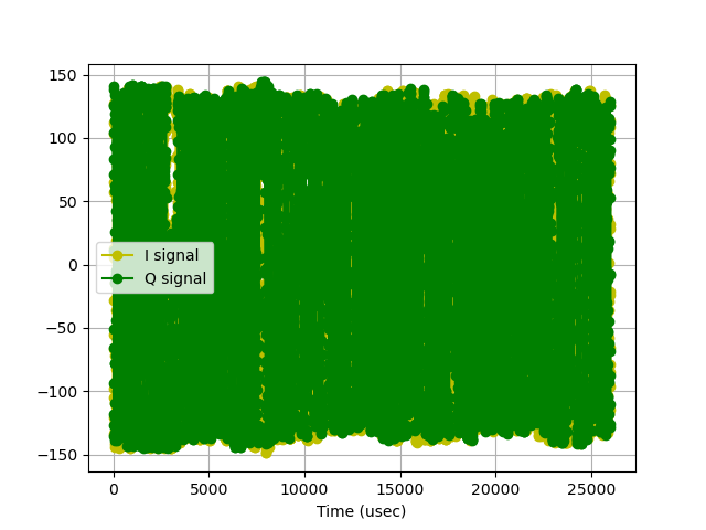
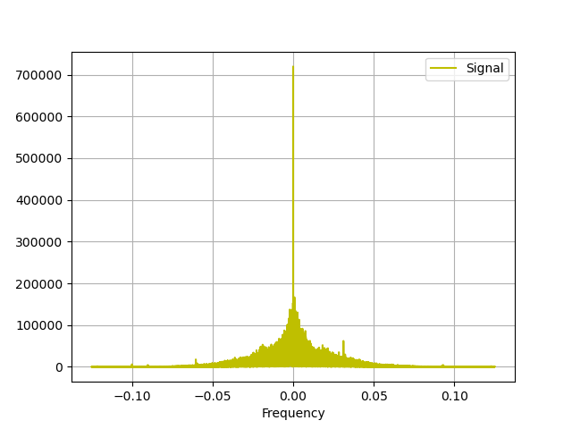
You may also notice that the super-structured side-bands that showed up last week are not as present. This is likely due to the somewhat aggressive rolloff of our CIC filters in hardware. We may have clipped out too much of the FM spectrum getting our sample rate down to 250 ksps. Oh well, this could be fixed later.

Now what we're still looking at is the Frequency-Modulated signal. It would be nice to demodulate this. We can do that in software by doing this (line to uncomment):

c_data = 0.5*np.angle(c_data[0:-1]*np.conj(c_data[1:])) #demodulate

Then run again.

Wait. How the Aitch-Eee-Double-Hockey-Sticks does that do demodulation? So:

If you have an incoming complex signal (which we do have from our IQ sampling):

s[t] = A\cdot e^{j\left(\omega_c + \omega_m\right)t}

where t is time A is the signal amplitude, \omega_c is the carrier frequenc (2\pi f_c) and \omega_m (2\pi f_m) is our information signal (this is F_M_ after all), then we want to isolate that signal.

Now the value for \omega_c at this point in the signal path is 0 since we already multiplied it by the carrier and did one of those \omega_c-\omega_c terms with some isolation (one of the side effects of our downsampling and filtering earlier on. As a result the IQ data coming in at this point is "carrier-frequency-independent" and is more appropriately expressing a signal that is :

s[t] = A\cdot e^{j \omega_m t}

Since \omega_m t is just a time-varying phase, we could say that the signal at any point in time is also just an expression of:

s[t] = A\cdot e^{j \phi_t}

What can be done to do this is to multiply the signal at one sample point by the complex conjugate of the signal one sample earlier, in effect doing a discrete time derivative on complex phase. So:

s[t_1]\cdot s^*[t_2] = A\cdot e^{j\phi_{t_1}} \cdot A\cdot e^{-j\phi_{t_2}}

Now when two exponents are multiplied, the stuff in their up-top gets added so the new signal is:

s[t_1]\cdot s^*[t_2] = A^2\cdot e^{j\left(\phi_{t_1}-\phi_{t_2}\right)}

That change in phase between two time steps \left(\phi_{t_1}-\phi_{t_2}\right) is going to be based solely on the whatever the frequency was multiplied by the duration of the timestep. Because our sample rate is fixed, that means that the whatever the angle of that complex value is, is directly proportional to our frequency...and the only frequency present now is our modulation frequency...so whatever the angle is that is our frequency The frequency over time is our signal so we've actually recovered (demodulated) our signal!

So we find the angle of this complex value and that is the signal demodulated!

With that demodulation done your time-domain signal will look different but still kinda hard to understand... but you should start to see more obvious amplitude variations since we're not longer looking at FM (which should have a constant amplitude with varying frequency), but now instead our original signal which will have amplitude and frequency variations!

More cool, though is that the frequency domain now should show the true composition of a commercial FM station's transmission in all its glory:

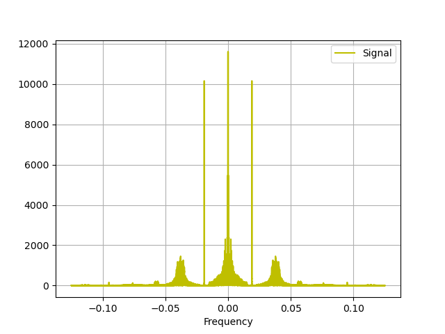
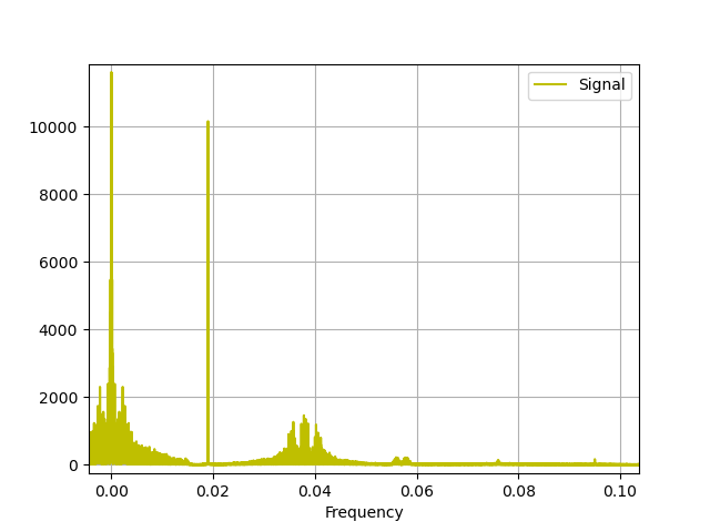
And zooming in we can see:

The low frequency information containing audio (L+R channel)
The 19 kHz pilot tone used to indicate the presence of stereo audio (L-R) signal centered around
The stereo signal (L-R) centered around 38 kHz
The small pile of signal about 4 kHz in bandwidth around 58 kHz which is the digital data listing the song-track and things about the station (final project idea maybe???)

SICK.

Each of these portions can be isolated and worked with.

OK audio is fine to look at, but it is even better as audio. Here's this script which is basically the same as before except instead of plotting we're making an audio file.

There are a few extra lines...the signal we care about (from above) for today is just the non-stereo audio around the 0 kHz base...we'll run a low-pass-filter on it with a cutoff of 6.25 kHz to remove everything we don't want. Then we'll decimate yet again (a third time) to 12.5 ksps. Then we'll have Python make an audio file for us.

import numpy as np
import time
%matplotlib notebook
import matplotlib.pyplot as plt
from pynq import allocate
from scipy.signal import firwin
from IPython.display import Audio
# Sampling frequency
#fs = 147.456
fs = 0.25 #new for this week (250 ksps)
# Number of samples
n = 262134 #new for this week (maybe)
#n = 65536
T = n/fs
down_from_center = center_frequency - fs/2
up_from_center = center_frequency + fs/2
# Time vector in seconds
t = np.linspace(0, T, n, endpoint=False)
# Allocate buffers for the input and output signals
ns = np.linspace(down_from_center, up_from_center,n,endpoint=False)
out_buffer = allocate(400024, dtype=np.int32) #more than big enough to hold ~quarter million samples
# Trigger the DMA transfer and wait for the result
start_time = time.time()
dma.recvchannel.transfer(out_buffer)
dma.recvchannel.wait()
stop_time = time.time()
hw_exec_time = stop_time-start_time
print('Hardware execution time: ',hw_exec_time)

imag = np.array([np.int16(out_buffer[i]&0xFFFF) for i in range(n)])
real = np.array([np.int16(out_buffer[i]>>16) for i in range(n)])
out_buffer.close()
c_data = real + 1j*imag #make complex data
c_data = 0.5*np.angle(c_data[0:-1]*np.conj(c_data[1:]))
taps = firwin(numtaps=101, cutoff=6.25e3, fs=250e3) #make another anti-alias filter for 20X decimation
c_data = np.convolve(c_data, taps, 'valid') #apply filter!
c_data=c_data[::20] #downsample to 12.5 ksps (factor of 20)
Audio(data=c_data.real, rate=12.5e3) #make audio signal at 12.5 ksps (use real component)

When this runs a little audio-player should pop up afterwards. With headphones in, press play. You should hear a one-second clip of audio from whatever station you were targetting. Sick.

Now...we just did a lot of our signal pipeline in Python to prove that there was a signal there. Your mind should immediately be going to what things that we just did (that were slow in software) could we do in hardware? And the answer is basically everything...

I mean:

The demodulation step could be done...especially the np.angle part...hello? CORDIC?
The final anti-aliasing step to get to 12.5 ksps audio
Even the audio generation itself...maybe you don't sent it to Python but instead make a PWM or PDM signal and send that out to speakers.

The possibilities are endless.

Lab 7 Checkoff:
Show your working RFSoC system

Footnotes

¹why didn't we do that last week? Honestly, I didn't realize I could make 64 MHz work with this. I had to futz around with the sample rates and decimation factors a bit to figure that this would work out. Next year we'll just directly do this in the previous lab. Oh well. (click to return to text)