The Setup

OK the goal today is to spin up the RFSoC. There are a few out at certain lab stations. No food at those lab stations. Most of what you're doing is going to be the same as if you were on the Pynq Z2 board so definitely make sure to refer back to those notes/pages.

Go in and make a new project just like before. Insteady of choosing the Pynq board, choose the RFSoC 4x2 board which you should have as an option on the lab machines. Click through everything else as before.

We don't need much of an XDC file for what we're doing but sometimes having some switches and LEDs is nice for sanity-check debugging. Use this below to make your XDC file:

## USER LEDS
set_property PACKAGE_PIN AR11 [ get_ports "led[0]" ]
set_property IOSTANDARD LVCMOS18 [ get_ports "led[0]" ]

set_property PACKAGE_PIN AW10 [ get_ports "led[1]" ]
set_property IOSTANDARD LVCMOS18 [ get_ports "led[1]" ]

set_property PACKAGE_PIN AT11 [ get_ports "led[2]" ]
set_property IOSTANDARD LVCMOS18 [ get_ports "led[2]" ]

set_property PACKAGE_PIN AU10 [ get_ports "led[3]" ]
set_property IOSTANDARD LVCMOS18 [ get_ports "led[3]" ]

## USER SLIDE SWITCH
set_property PACKAGE_PIN AN13 [ get_ports "sw[0]" ]
set_property IOSTANDARD LVCMOS18 [ get_ports "sw[0]" ]

set_property PACKAGE_PIN AU12 [ get_ports "sw[1]" ]
set_property IOSTANDARD LVCMOS18 [ get_ports "sw[1]" ]

set_property PACKAGE_PIN AW11 [ get_ports "sw[2]" ]
set_property IOSTANDARD LVCMOS18 [ get_ports "sw[2]" ]

set_property PACKAGE_PIN AV11 [ get_ports "sw[3]" ]
set_property IOSTANDARD LVCMOS18 [ get_ports "sw[3]" ]


set_property BITSTREAM.CONFIG.UNUSEDPIN PULLUP [current_design]
set_property BITSTREAM.CONFIG.OVERTEMPSHUTDOWN ENABLE [current_design]
set_property BITSTREAM.GENERAL.COMPRESS TRUE [current_design]

When ready, make a new block diagram design. Don't click automate/wiring until you've got all your pieces laid out.

We need to add some things:

The Processor

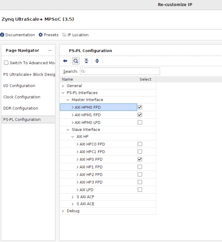
Make a processor like before. This will be fancier than the Zynq Series 7 one, but effectively the same thing, just with more options. We'll need two HP Master ports (one for the ADC and one for the DMA) and then and one HP Slave port (for the DMA). I made them all 128 bits in size. That should be fine. We can worry about optimizing that later. Details below:

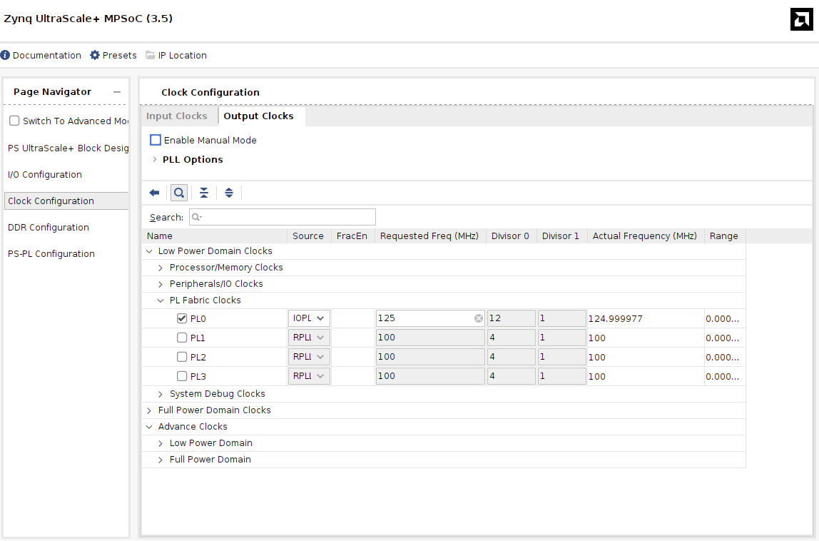
Also under the clocks/output-clocks tab, make sure you have peripheral clock specified like shown below:

The DMA module

The DMA can be very simple (just like before). This will require one fresh DMA. We're not going to be reading from the DMA (from the perspective of the PL, mind you), only writing...so we only need a write channel. Settings I used below are shown. Make sure scatter-gather is disabled, though that probably doesn't matter (but I haven't tested it).

RF Data Converter

OK now we need to add the new thing. The RF Data Converter. Search for that when you add it, customize it like shown in the two figures below.

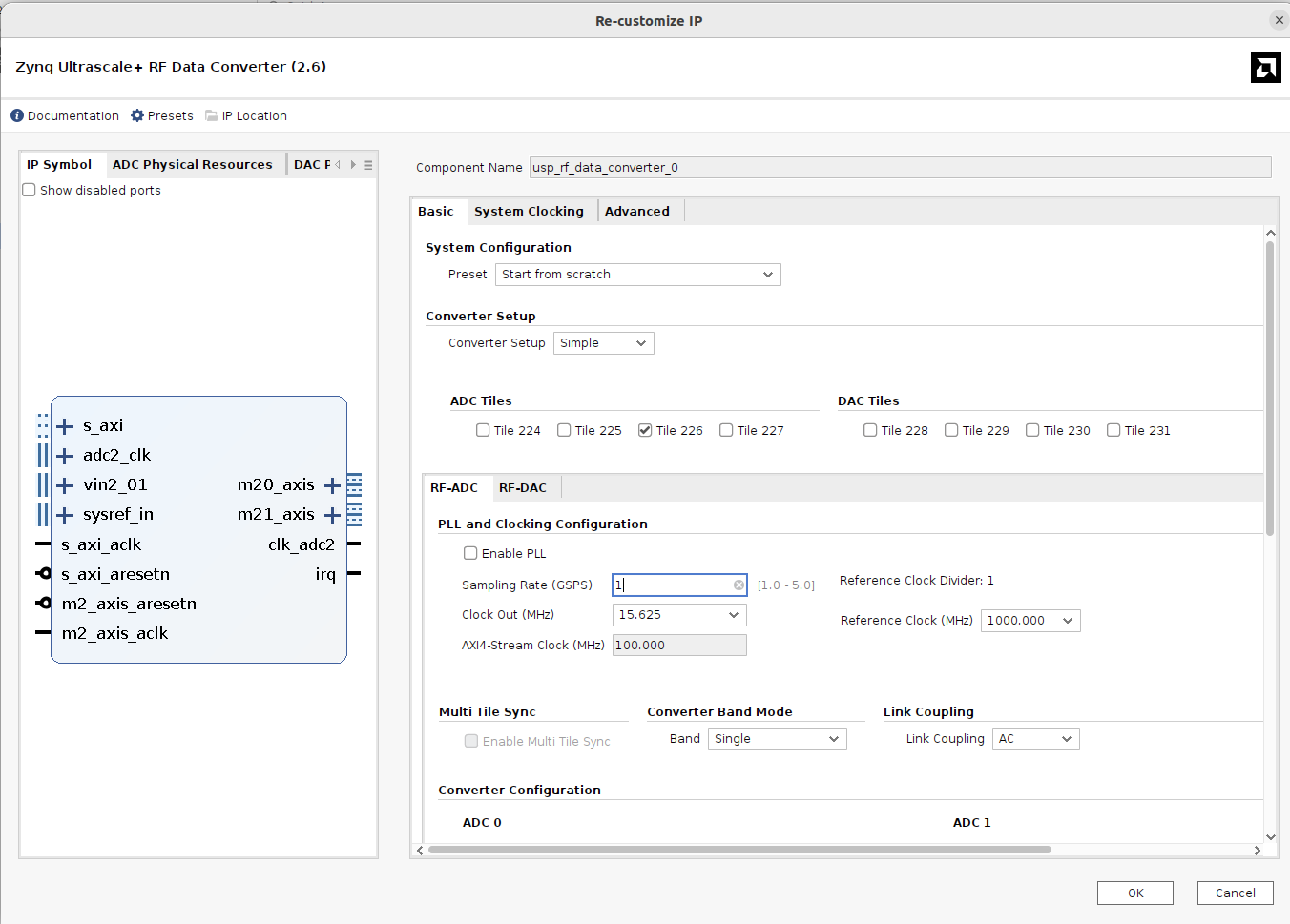
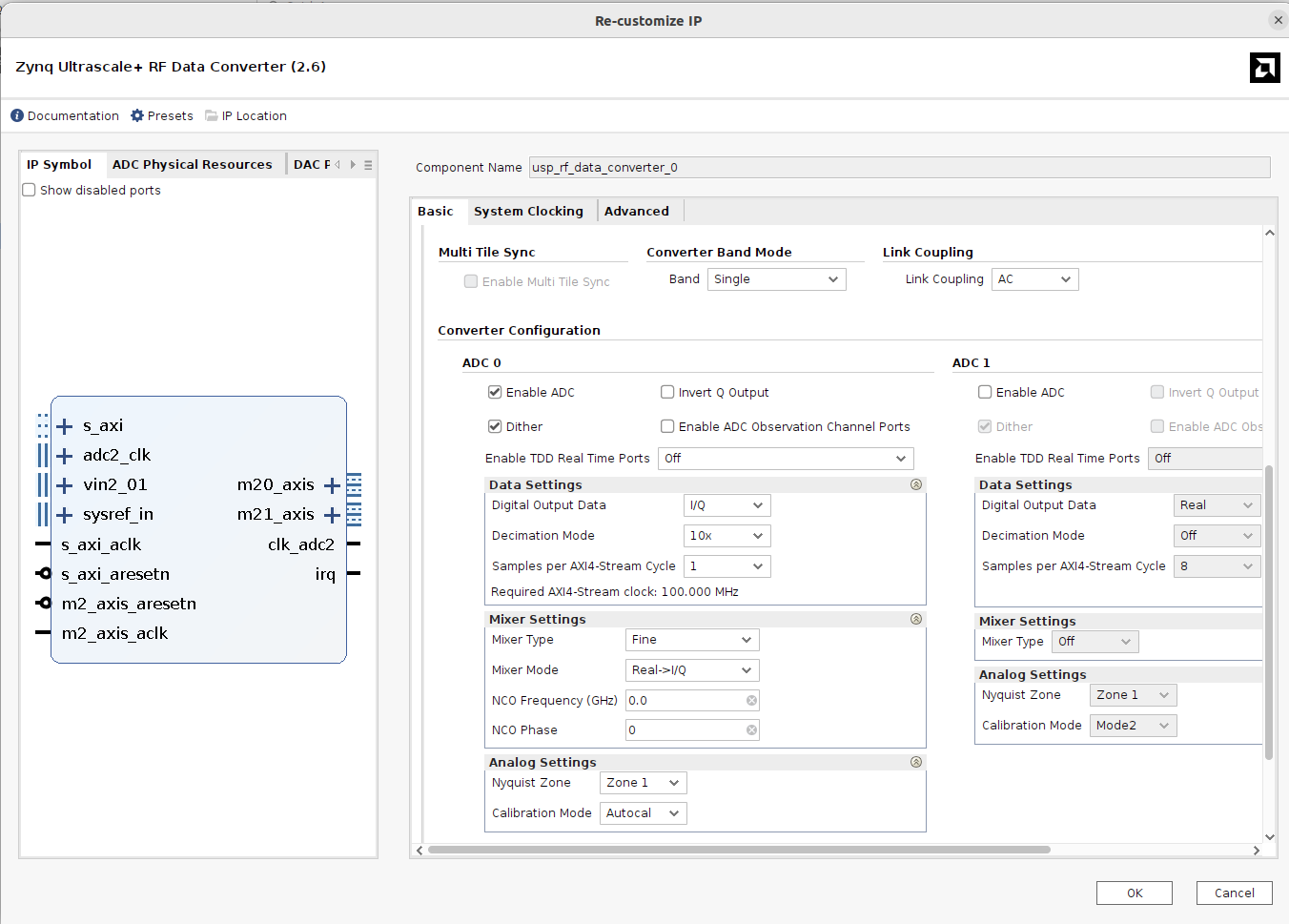
We're essentially (I thought anyways), telling this thing to sample at 1 Gsps, do quadrature/complex down-mixing (At a frequency will be able to set from Python), and then read out the data. For whatever reason, this thing seems to be setting the sample rate slightly wrong (factor of two off in the low direction), so the signals we end up capturing appear to be 2X in the frequency space. I'm still not sure what is causing this...I'll talk more about this later on. But for now these settings will work for the moment (I may change this once I figure out what the h is going on. I'm probably just being stupid). After the quadrature mixing, the signals are then decimated by a factor of ten (with appropriate anti-alias filtering between done automatically) so that we'll have 100 Msps per second.

For high sample rates, you'll need to send out multiple samples at a time in an ever-widening bus. To keep things simple for today, let's just pick numbers that allow us to get 1 sample per clock cycle at 100 MHz.

Anyways this newly configured piece of RF grabbing IP should look like this:

A Piece of IP You Must Make

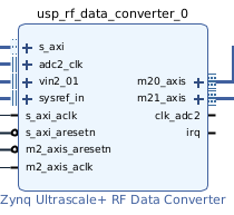
The RF Data converter will work as it is, but without any context/packaging, it is tough to get it into the PS side. As a result, there's a few things we want to do to "package" the data stream coming out of the DDC. We'll wrap all of that functionality up into a single piece of IP which I'll call "TLAST_maker", but you can call it whatever you want. This piece of IP will live between the RF data converter and the DMA. All of its ports are shown fully-expanded out:

This thing has to do primary tasks:

Task 1: Merge Channels

The output of the DDC as configured will produce two independent AXI Streams containing the I and Q data from the complex down-mixing. This is a weird choice in my opinion since an I/Q pair of values really should move through life together...and adding to the mystery, each I/Q value is signed 14 bits so you could easily fit both in a stacked format within a standard 32 bit AXI Streaming data channel , but who am I to question. Instead the I and Q values come out in two non-standard 16-bit AXIS busses, complete with their own READY and VALID signals, etc...

To get them into the DMA we need to merge them together into one channel, (or alternatively we could have two DMA blocks with each written to that...but the DMA needs to be 32 bits I believe...so then you'd be running at 50% bandwidth efficiency...)...so we'll just instead merge our two streams into one 32 bit stream.

The data sheet (taken from here) implies that both channels are perfectly synchronized and in my testing this seems to be the case (which further adds to the mystery of why not putting them in one stream in the first place, but whatever).

So we need to make this piece of custom AXI streaming IP take two AXI slave ports and merge them together with this in mind. The fact that they are perfectly synchronized means you can just use both valid signals together to decide when to sample both and then just feed the TREADY back pressure signal back through one module and call it a day. In a real AXIS-merging device you'd have to do some fancy cross-checking logic to deal with the unsynchronized issues of the two input streams, but that doesn't seem to be needed here.

So I took my two measurements I/Q values and stacked them...I on the lower 16 and Q on the top 16. This should be good enough for this lab.

Task 2: TLAST

The second big issue is that the data which comes out of our RF data converter will just be sample after sample with no context or framing to them. Unfortunately, we can't just feed this data stream into a DMA Slave AXIS port because there's no TLAST signal on it...which means when you try to read/wait for the DMA write transation to take place, you'll hang forever (think back to the FIR stuff you worked on and the bugs with that). We need to add a TLAST signal to it. This is going to be basically the simplest framing we can. For this I used an internal counter capable of counting up to 262143 (2^18-1). Based on the input values of the control signal (which I tied to my switches), a TLAST signal would fire either every 65536 samples or 262144 samples. As a result, we just repeatedly and periodically send in transfers of data that are "framed" with the TLAST signal.

In practice the DMA is not always ready to read, so it will normally, when we're not prompting it in python, hold up the show, and that's fine with this...the ADC samples will just get lost, but we have nowhere to put them anyways. But when we do go in and do a READ as long as we tell the DMA transfer to be a size larger than 262144 measurements (4 bytes per measurement), because what we're writing to memory via the DMA will be smaller than that python won't hang...it'll be guaranteed to get a TLAST signal in within that wait period.

So build that piece of IP (it should be pretty simple and I'd honestly just suggest writing it in regular Verilog in the top-level of the IP you create (delete those default Master/Slave Stream bus managers it puts in there).

I added a 4-bit input for debugging and TLAST/burst setting as well as a 4-bit output (That I connected to LEDs during my debugging) as well.

Make sure to change the width of your two AXI Slave ports to 16 bits...else you won't be able to match them to the outputs from the RF Data converter.

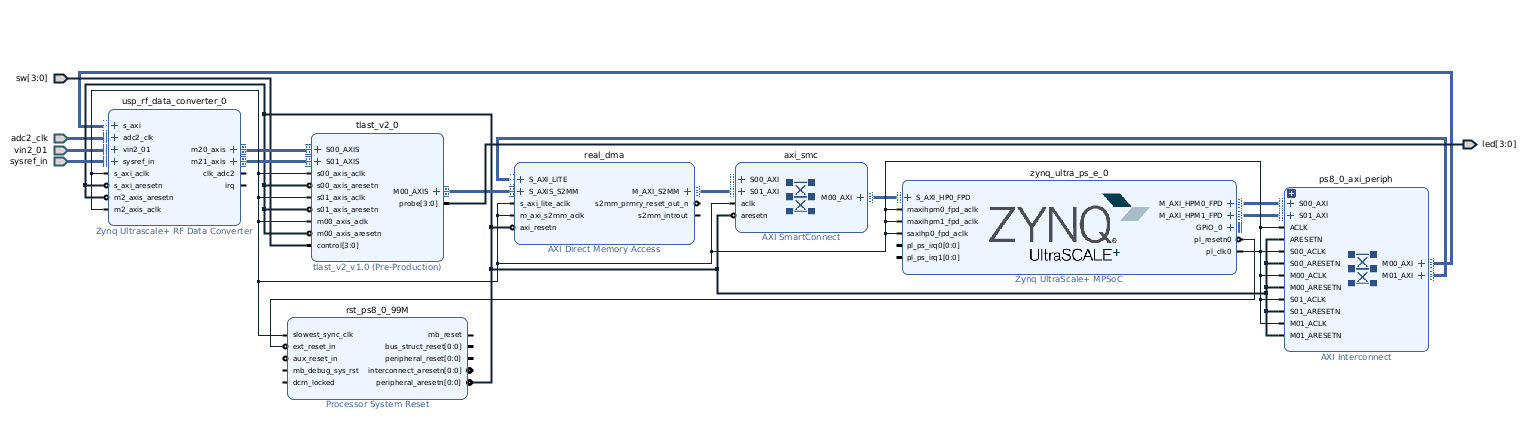
Wire it All Up

Ok with these pieces all laid out, go ahead and route the AXI Streaming portions...

• RF Data Converter to TLAST_Maker
• TLAST_Maker to DMA

Once that is done, go ahead and let Vivado try to wire things up for you. That might take a couple of runs/wirings. You may also need to move components around and then do the prettify buttons to get the wires and busses in clean-to-read orientations¹

My layout looks like the following:

When ready, go ahead and build and everything like before.

You need to add a license to your Vivado in order to build. Here are the license files for machines 19-30 in the lab:

• machine 19
• machine 20
• machine 21
• machine 22
• machine 23
• machine 24
• machine 25
• machine 26
• machine 27
• machine 28
• machine 29
• machine 30

Put on the Board

OK Now it has to go onto the RFSoC. You need a fresh/new SD card for this. I have them at the front in special little holders for you.

Put one into an available, RFSoC, power it on, let it boot up (it'll take a minute or two) and when it is completed, the OLED in the middle will display the IP Address of th eboard (omg the luxury).

You should be able to just go to that IP address and find the device on the network just like before.

Upload the hardware handoff file and the bit file like before.

Then let's make a new notebook.

First let's do the old regular stuff (load the bit file/overlay, etc.)

from pynq import PL
PL.reset() #important fixes caching issues which have popped up.
import xrfdc #poorly documented library that handles interfacing to the RF data converter
from pynq import Overlay  #import the overlay module
ol = Overlay('./design_1_wrapper.bit')  #locate/point to the bit file
import pprint
pprint.pprint(ol.ip_dict)
dma = ol.real_dma #might need to change name depending on what you called it
rf = ol.usp_rf_data_converter_0 #might need to change name depending on what you called it

The last two lines grab handles to constructs we've created. The DMA you know and love already. The RF one is a handle to our RF converter. We can study and manipulate its settings as needed.

The ADC we activated is on the third ADC tile ("226" or index 2) and is the first tile (index 0). We need to grab a software handle to it and check its status.

adc_tile = rf.adc_tiles[2]
print(adc_tile)
adc_block = adc_tile.blocks[0]
print(adc_block)
print(adc_block.BlockStatus)
print(adc_block.MixerSettings)
adc_block.Dither = 0 #doesn't really matter for this lab, but let's turn off.
adc_block.MixerSettings['Freq']= 0 # set the frequency of the Numerically controlled oscillator.
adc_block.UpdateEvent(xrfdc.EVENT_MIXER) #every time setting is changed, must call this.
print(adc_block.MixerSettings)

For starters

import numpy as np
import time
%matplotlib notebook
import matplotlib.pyplot as plt
from pynq import allocate

def plot_to_notebook(time_sec,in_signal,n_samples,):
    plt.figure()
    plt.subplot(1, 1, 1)
    plt.xlabel('Time (usec)')
    plt.grid()
    plt.plot(time_sec[:n_samples]*1e6,in_signal[:n_samples],'y-o',label='Input signal')
    #plt.plot(time_sec[:n_samples]*1e6,in_signal[:n_samples],'y-o',label='Input signal')

    plt.legend()
def iq_plot(time_sec,re_signal,im_signal,n_samples,):
    plt.figure()
    plt.subplot(1, 1, 1)
    plt.xlabel('Time (usec)')
    plt.grid()
    plt.plot(time_sec[:n_samples],re_signal[:n_samples],'y-o',label='I signal')
    plt.plot(time_sec[:n_samples],im_signal[:n_samples],'g-o',label='Q signal')
    #plt.plot(time_sec[:n_samples]*1e6,in_signal[:n_samples],'y-o',label='Input signal')

    plt.legend()

def plot_fft(samples,in_signal,n_samples,):
    plt.figure()
    plt.subplot(1, 1, 1)
    plt.xlabel('Frequency')
    plt.grid()
    plt.plot(samples[:n_samples],in_signal[:n_samples],'y-',label='Signal')
    #plt.plot(time_sec[:n_samples]*1e6,in_signal[:n_samples],'y-',label='Signal')
    plt.legend()

# Sampling frequency
fs = 100
# Number of samples
n = 65536
T = n/fs

# Time vector in seconds
t = np.linspace(0, T, n, endpoint=False)
# Allocate buffers for the input and output signals
ns = np.linspace(0, fs,n,endpoint=False)

out_buffer = allocate(400024, dtype=np.int32)
# Trigger the DMA transfer and wait for the result
start_time = time.time()
dma.recvchannel.transfer(out_buffer)
dma.recvchannel.wait()
stop_time = time.time()
hw_exec_time = stop_time-start_time
print('Hardware execution time: ',hw_exec_time)

real = []
imag = []
#extract the two values (I and Q) from each 32 bit write from the hardware side.
for i in range(65536):
    val = out_buffer[i]&0xFFFF
    if val>=32768:
        real.append(np.int32(0xFFFF0000|val))
    else:
        real.append(val)
    imag.append((out_buffer[i]>>16))

# plot_to_notebook(t,real,6500)
# plot_to_notebook(t,imag,6500)
iq_plot(t,real,imag,6500)
c_data = np.array(real) + 1j*np.array(imag)
z = np.fft.fft(c_data,n)
plot_fft(ns,abs(z),65535)
out_buffer.close()

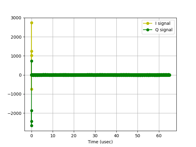
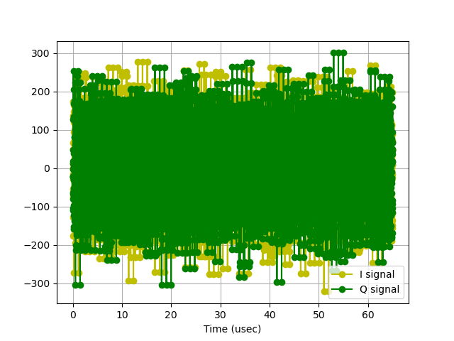
Now if you go and run this code you'll get a time plot of this (or something similar):

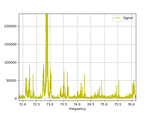
And a frequency plot of this:

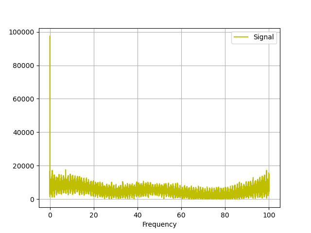
OK you've measured basically nothing and seen nothing. While not exactly a result that will win a Nobel Prize, it at least should hopefully check out. Is there anything out there that we could measure? Why yes, let's jam an antenna on and see if we can capture a signal out of the ether. Aroudn lab there should be some FM antennas that look like this:

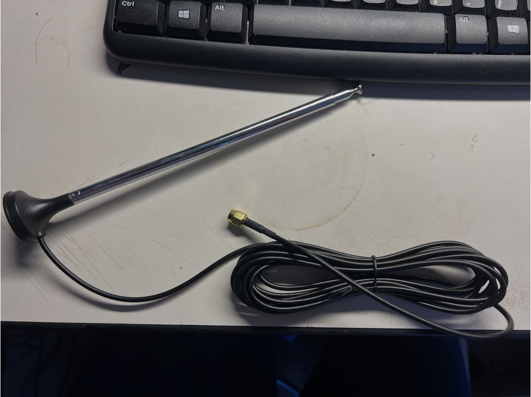
Grab one and attach it to ADC_B on the RFSoC. Commercial FM lives in the 88 MHz to 108 MHz frequency band. Our current effective ADC output sample rate is 100 Msps. This means there's no hope of getting that signal within our sample rate. But we do have a complex mixer at our disposal. We can set that things frequency to be a value that will then mix with our incoming signals to move that band down. (based on the f_s\pm f_m math we've talked about in class).

For a mixer frequency we'd want to pick something in the FM band on near there. 85 MHz might be a good choice. Since it would move the entire FM band down to base band and could easily fit within 100 MSps bandwidth. To do this you could try this.

adc_block.MixerSettings['Freq']= 85
adc_block.UpdateEvent(xrfdc.EVENT_MIXER) #every time setting is changed, must call this.

And then re-run but it won't work. And this is getting back to the bug that I'm not sure about. The signals we are putting in are getting sampled at half the rate they should be. As a result, signals are appearing at twice the frequency one would expect. So when we try to mix down using 85, we're actually not targeting the right frequency space. Instead we need to double our mixing frequency:

adc_block.MixerSettings['Freq']= 170
adc_block.UpdateEvent(xrfdc.EVENT_MIXER) #every time setting is changed, must call this.

Now rerun and you should see something like this:

Suddenly...there is signal where there was none. We've pulled FM down into our baseband window.

And a frequency plot looks even cooler...

Zooming in on one of the large spikes you can actually see a complete FM commercial station in the frequency space. You may notice lots of "clones" of the large signals going out in both directions...those are windowing artifacts which we could suppress with proper filtering...another day. It is actually kind of funny, the baseband of this RFSOC is so large, we're actually getting windowing artifacts of entire FM stations replicated out to either side. Some windowing would certainly go a long way to fixing that.

Since not everyone in the year of our lord 2024 knows what an FM station looks like in frequency space, here is a screengrab of one off of one of my Software Defined Radios.

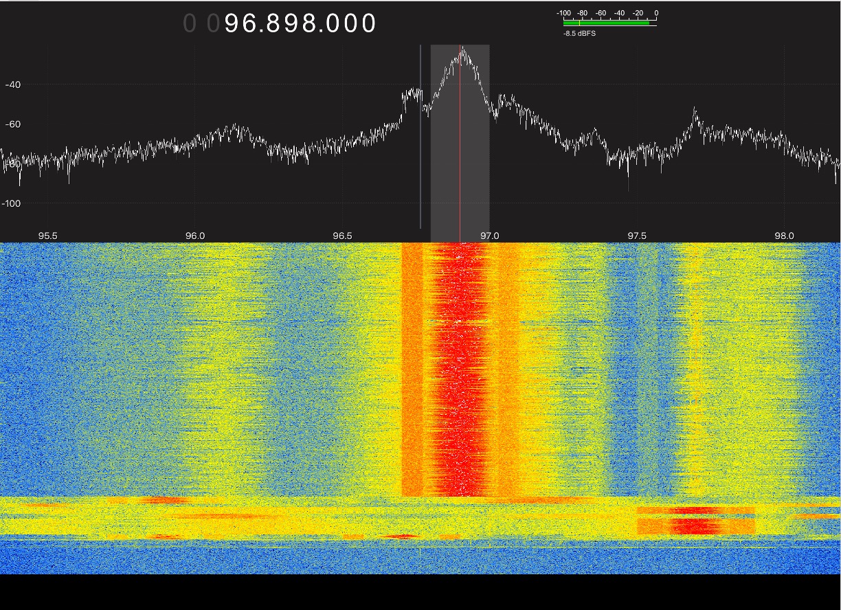
The fact that we can see this signal raw is a testament to the strength of commercial FM stations (there are transmitters literally across the river on the top of the Prudential Building).

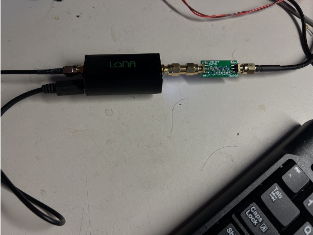
If we wanted to improve our signal-to-noise we should amplify and target our signal more. To do this, I have a couple Low-Noise-Amplifiers and a few FM-band-pass filters in lab. Connect the antenna to the input of the LNA, the output of the LNA to the input of the filter, and then the output of the filter to ADC_B. Make sure the LNA is powered...

I only have a few of these filter ankk13

Re run and you should have much larger signals that are much, much further above the noise.

And a frequency plot looks even cooler... (again ignore the windowing artifacts of repeated clones)

Zoomed in, that is a good station.

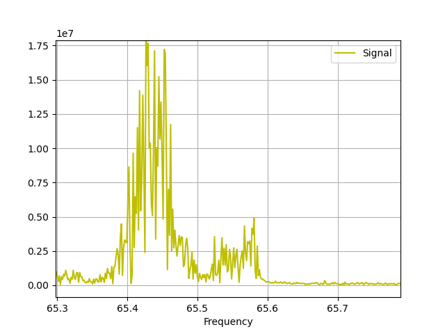
Note the FM band is shown 2X stretched here. This is another result of something not lining up with our sample rate. I'll get to the bottom of this eventually (or maybe you will)...but the info is there anyways!

Upload a zip of your working hdl files.

Select File No file selected

Ask for Help Loading...

Upload Some images of the FM space.

Select File No file selected

Ask for Help Loading...