Streaming FFT

Implementing a Streaming FFT

On this page we'll quickly go over building a full DMA-accessible FFT pipeline. This is going to reuse a good chunk of last week's streaming pipeline infrastructure, so please refer back to those notes and things.

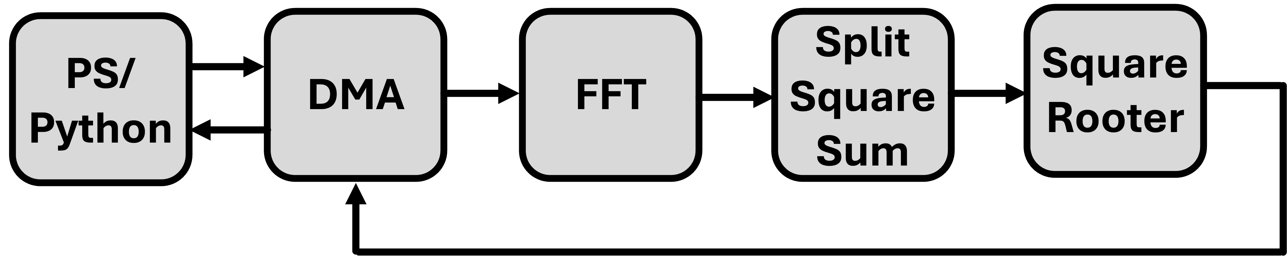
The system will involve a DMA interface to take in some time-series data, an FFT, some follow-up modules to figure out the magnitude of the FFT output, and then a return to the DMA interface. You should have already written and somewhat verified the module that "extracts" the complex numbers as well as the module that computes the square root.

Getting Started

Basically same startup as last week. Make a new project for the Pynq board. Make sure to target the Pynq board. Use your standard .xdc file. that you have been using. Create a new block diagram, add in a Zynq Processing System, and run the default automation. Bring in the DMA like last time, make sure to disable scatter-gather, and make the depth maybe 23 bits, again like last time.

The FFT

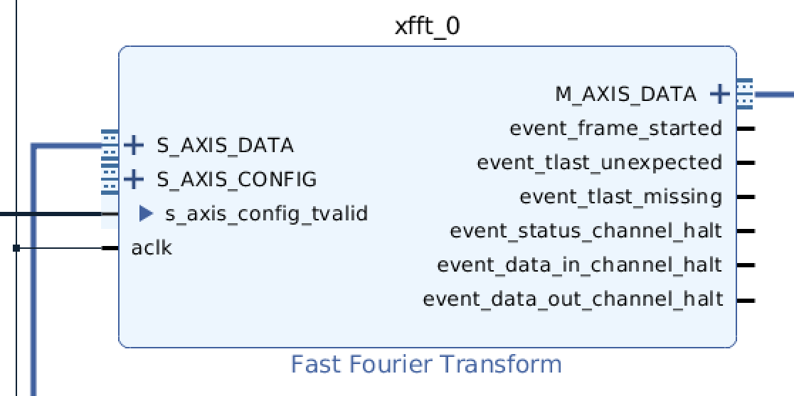
The new kid on the block this week is the FFT so let's add it. Find it and go ahead and add it to your block diagram like shown below. Really the only input we'll use is the AXI Stream In, and the only output we'll be using is the AXI Stream Out.

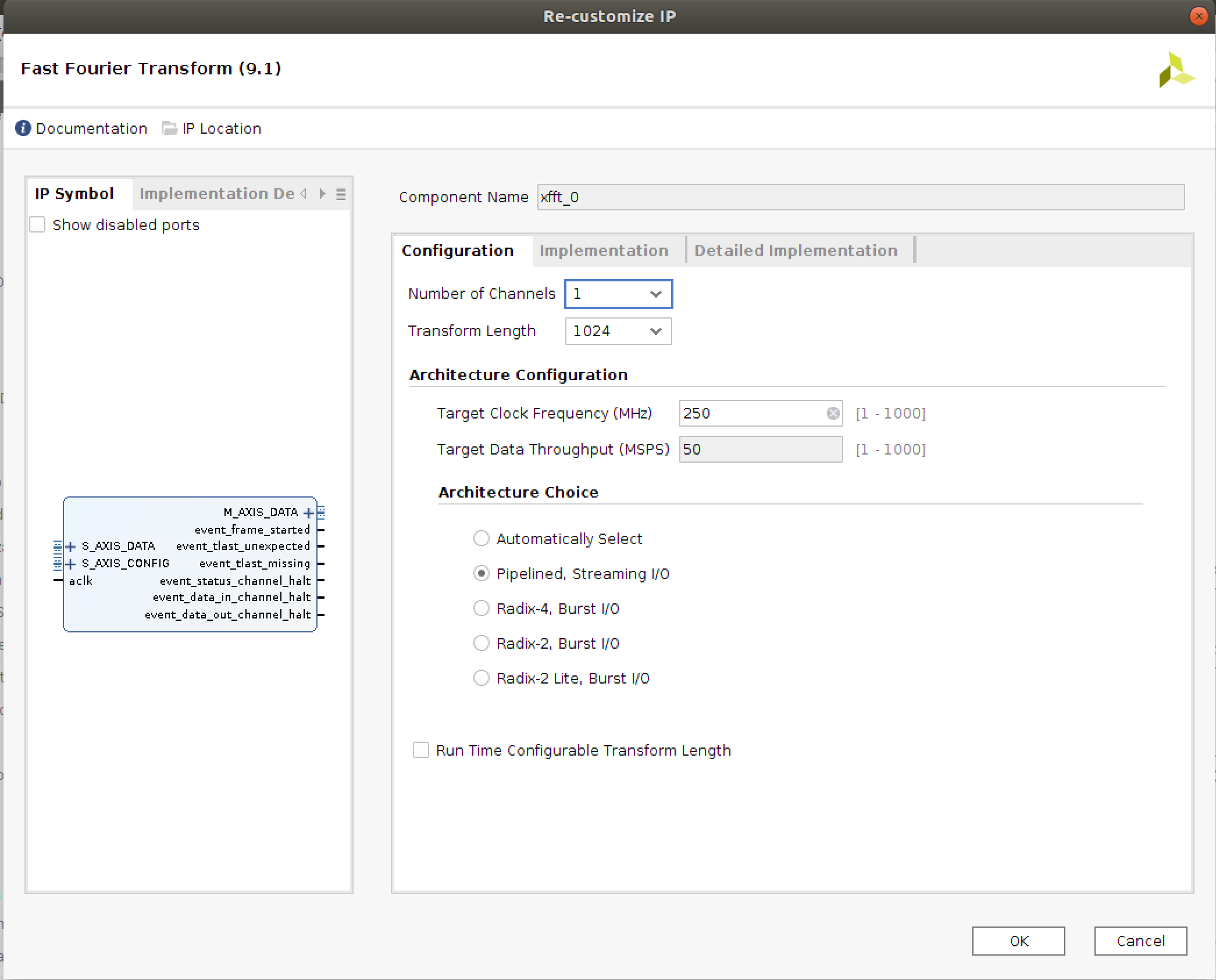
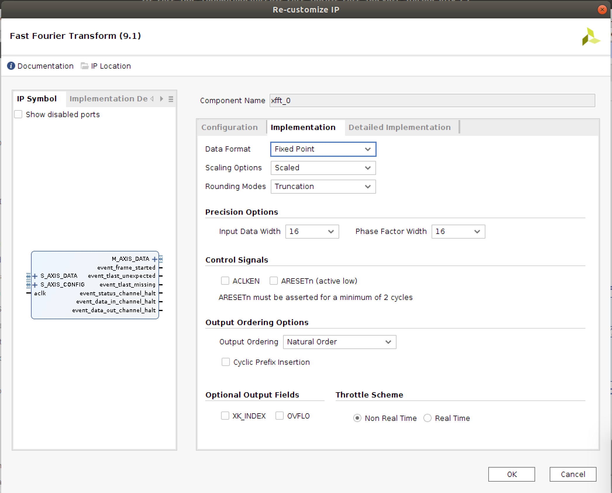
Set up your FFT so that it is for 1024 points, and the output values are in Natural Order among other things. This is important. If you don't do it, the values will come out in the algorithmically most efficient manner, which is actually not in the order of spectral components. Most of the settings should stay the same, but please compare to the images below:

After you've added it, connect its AXI4 Streaming Input to the AXI4 Streaming Output of the AXI-DMA module.

To avoid an error, add a Constant IP with value of 0 to the design and tie it to the s_axis_config_tvalid input on the FFT just to suppress an inevitable error that will pop up about some undefined input. The Constant can be added in the block diagram like any other piece of IP.

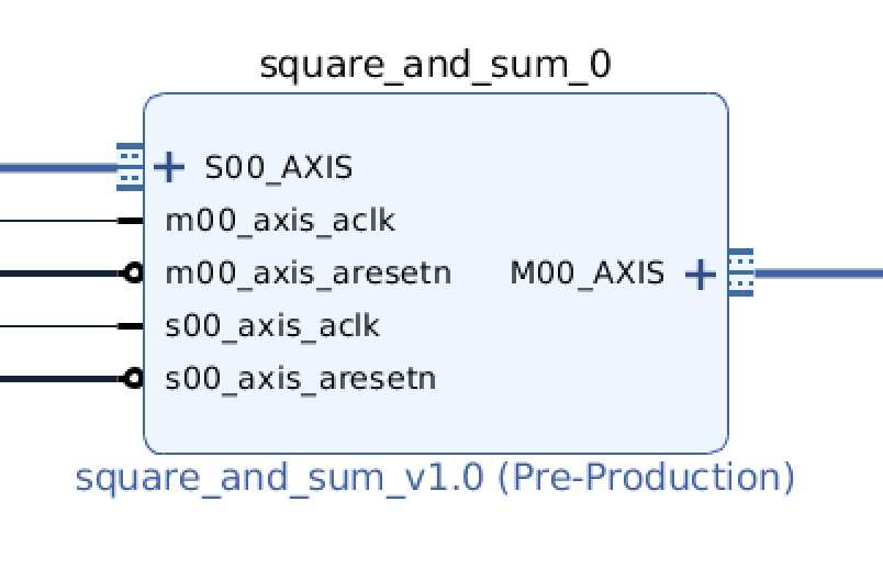
Split-Square-Sum

Now we need a module to the take the complex output of the FFT and turn that into a magnitude (since that's all we care about for this lab...in other applications you may very well want to keep the real and imaginary part separate). You already wrote the module to do this. Just like last week, create a new piece of streaming AXI IP and incorporate your module that takes the pair of 16 bit real and imaginary values and splits, squares, and sums them.

Square-Rooter

Do the same thing for your square-root calculator. If you'd like to merge both modules (split-square-sum and square-rooter) into one single piece of "IP" totally feel free to do so. I'll leave that up to you. Just make sure you have both files in included (but not copied) in the same IP module so you can use them together.

Once your code is done, DON'T FORGET TO REPACKAGE THE IP and add a copy to your high level block diagram. Wire the output of the FFT to its input.

AXI Streaming FIFO

If you want (you don't need to, but just to get more practice), feel free to add an AXIS FIFO Now let's add a AXI Streaming FIFO between the output of your square root module and the input to your DMA. We actually probably don't need this here, but I wanted to add this here just so you know it is a thing you can use as needed.

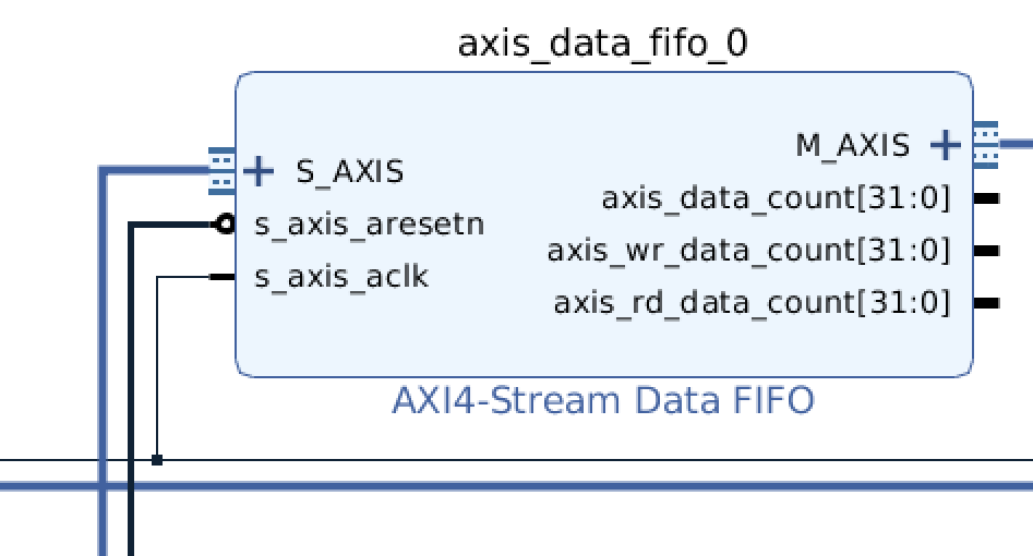
I believe that we'll use most of the default settings as it comes, but double-check below. The Width needs to change, for example.

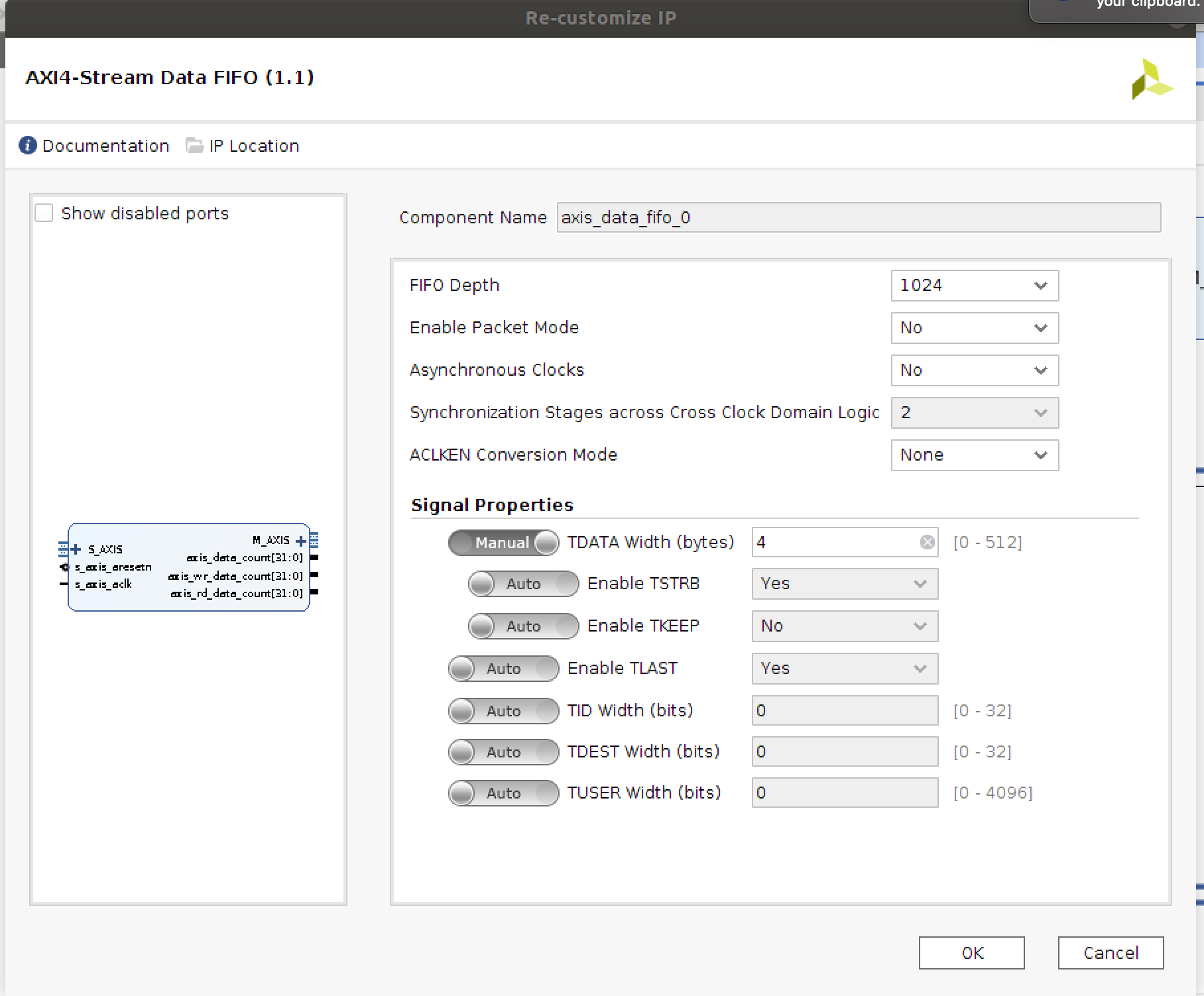
In order to make this module perfectly compatible with our AXI4-Streaming pipeline, make sure the T_LAST and TREADY and TSTRB signals are activated:

Wiring It All Together

At this point you should be able to wire everything up. Do the main pieces yourself (the AXIS connections) but then feel free to run the auto-wiring automation if it hasn't been done. Take care that Vivado has a tendency to deactivate the High speed Slave Port you activate in the Znyq core sometimes. Not sure why, but be on the lookout for that going away and then fixing it if it does.

If all looks good, go through your standard build process like you have been doing.

Interacting With It In Python

Once you've got your bit file and hwh file up in place, the snippets of code below should work with your module.

from pynq import PL
PL.reset() #important fixes caching issues which have popped up.
from pynq import Overlay  #import the overlay module
ol = Overlay('./design_1_wrapper.bit')  #locate/point to the bit file
import pprint
pprint.pprint(ol.ip_dict)
dma = ol.axi_dma_0 #change if needed.

import numpy as np
from scipy.signal import lfilter
import time
%matplotlib notebook
import matplotlib.pyplot as plt
from scipy.signal import lfilter

def plot_to_notebook(time_sec,in_signal,n_samples,out_signal=None):
    plt.figure()
    plt.subplot(1, 1, 1)
    plt.xlabel('Time (usec)')
    plt.grid()
    plt.plot(time_sec[:n_samples]*1e6,in_signal[:n_samples],'y-',label='Input signal')
    if out_signal is not None:
        plt.plot(time_sec[:n_samples]*1e6,out_signal[:n_samples],'g-',linewidth=2,label='Module output')
    plt.legend()
def plot_fft(samples,in_signal,n_samples,):
    plt.figure()
    plt.subplot(1, 1, 1)
    plt.xlabel('Frequency')
    plt.grid()
    plt.plot(samples[:n_samples],in_signal[:n_samples],'y-',label='Signal')
    #plt.plot(time_sec[:n_samples]*1e6,in_signal[:n_samples],'y-',label='Signal')
    plt.legend()

# Sampling frequency
fs = 100e6
# Number of samples
n = 1024#int(T * fs) 1024
#Total Time:
T = n*1.0/fs
# Time vector in seconds
t = np.linspace(0, T, n, endpoint=False)
ns = np.linspace(0,fs,n,endpoint=False)
# Samples of the signal
samples = 2000*np.cos(2e6*2*np.pi*t) + 1000*np.cos(10e6*2*np.pi*t) + 600*np.sin(20e6*2*np.pi*t) +0
samples = samples.astype(np.int32)
print('Number of samples: ',len(samples))


# Plot signal to the notebook
plot_to_notebook(t,samples,1024)
start_time = time.time()
z = abs(np.fft.fft(samples))
stop_time = time.time() #just after operation run
sw_exec_time = stop_time - start_time
print('Software execution time: ',sw_exec_time)

# Plot the result to notebook
# plot_to_notebook(t,samples,1000)
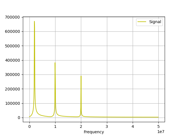
plot_fft(ns,z,512)
# #HARDWARE TIME
# #now it is time to run on hardware:
from pynq import allocate
# import numpy as np

# # Allocate buffers for the input and output signals
in_buffer = allocate(shape=(n,), dtype=np.int32)
out_buffer = allocate(shape=(n,), dtype=np.int32)

# # Copy the samples to the in_buffer
np.copyto(in_buffer,samples)

# # Trigger the DMA transfer and wait for the result
start_time = time.time()
dma.sendchannel.transfer(in_buffer)
dma.recvchannel.transfer(out_buffer)
dma.sendchannel.wait()
dma.recvchannel.wait()
stop_time = time.time()
hw_exec_time = stop_time-start_time
print('Hardware execution time: ',hw_exec_time)
print('Hardware acceleration factor: ',sw_exec_time / hw_exec_time)
# Plot to the notebook
plot_fft(ns,out_buffer,512)

# Free the buffers
in_buffer.close()
out_buffer.close()

When you run all this, you should first get a time-domain plot dependent on what you specify. For example, in the code it is currently set to the following, but please feel free to change it:

samples = 2000*np.cos(2e6*2*np.pi*t) + 1000*np.cos(10e6*2*np.pi*t) + 600*np.sin(20e6*2*np.pi*t) +0

In time that'll look like the following:

After that you'll get a hopefully correct FFT as an output! Actually you should get two of them...one from numpy's fft and one from your own FFT on the fpga. They should be similar in shape with peaks at the spot where you made signals in both of them. They may be different in scaling factors, though.

Once that is working, good. Upload your top level module and a couple screenshots of your notebook working.

Upload your inner verilog wrapper file (the one with all the module instantiations in it)

Select File No file selected

Loading...

Upload your inner verilog wrapper file (the one with all the module instantiations in it)

Select File No file selected

Loading...