The Setup

OK, you're an expert at this now. You need to make a new Zynq project. Go to Vivado, create a new project. Add in the base xdc file, pick the PYNQ Z2 board. Comment out all the xdc file. We actually don't need anything today other than DRAM, but we'll just put the XDC in, in case you want to expand on this later. So comment out the whole XDC.

Make a new block diagram and put in your processor. For this lab, wcan actually use it pretty much as is, except we want to enable one High Speed AXI Slave Port which will be used to Interface with the DMA which we'll add next.

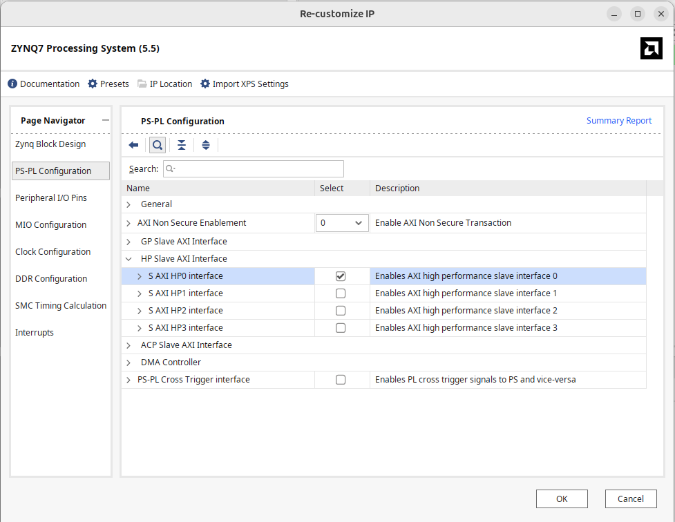
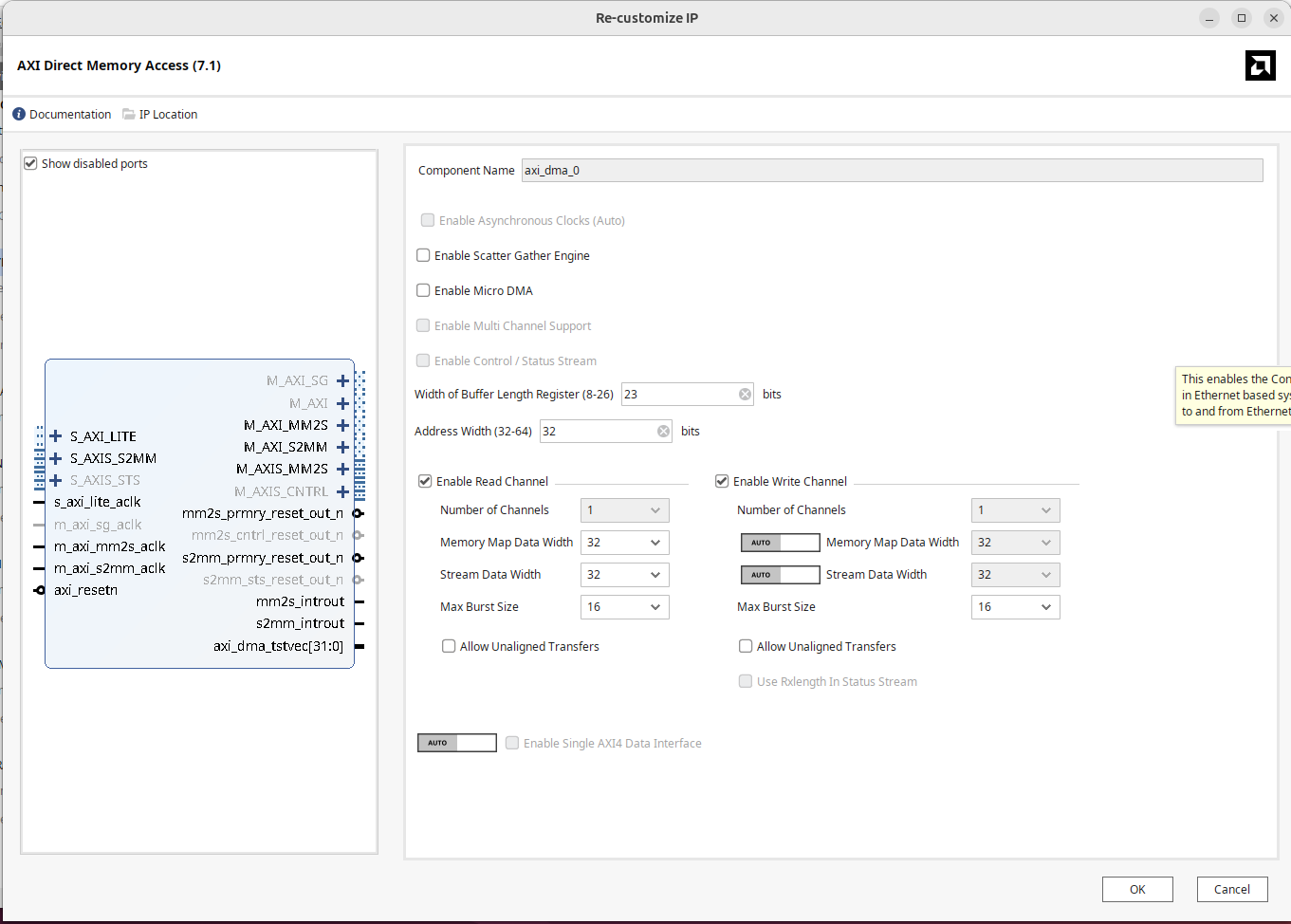
Next let's add a piece of IP called the AXI Direct Memory Access thing. (there's several "DMA" type IP's so make sure to add the correct one.) Once added, we need to configure it ever so slightly. Double click and in the settings window that comes up:

• Disable Scatter Gather (that's not enabled on this board)
• Set the width of the buffer length register to something like 23.

Otherwise leave everything as is...the settings should collectively look like the following:

Rename the DMA IP to dma rather than the automated name it creates. This will line up with the Python script later.

When done, don't do any automated wiring yet. Let's add in our third piece, the AXIS IP first. That way we don't need to tear up and redo.

The AXIS IP

Like last week, we're going to make a new piece of AXI IP.

1. Go up to Tools > Create and Package New IP
2. Click Next
3. Select Create AXI4 Peripheral
4. You can call it whatever you want, but I chose math_doer since we'll be doing some math (two different things).
5. In the next window that comes up it will show you a default module that has a single AXI4-LITE Slave Interface. And now we change from what we did last week...This is NOT what we want. We want two AXI ports...a Slave AXI Streaming and a Master AXI Streaming. Add/modify them until you have both of them. It should look like the figure below:

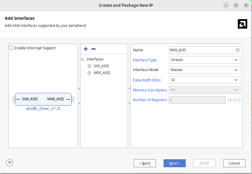
I'd just recommend adding your IP to your local IP repo when it prompts you, but you do you. When ready, go in and edit it.

Our Design

From the previous pages of work we should have a few functioning (hopefully) pieces of AXI streaming IP (the 3*x+100 one provided and then the FIR15 module you should have hopefully written). Both of these take in values on one side and poop them out the other side so they'll fit in perfectly with the AXIS IP we're making. If you open the default top file of the IP, there are going to be two generic skeletons controlling each port. What you're really supposed to do is write your own stuff to interact with these two modules who then handle all the AXI rules for you, but to be honest, AXI Streaming is so simple, and we're making systems that are relatively simple, that we can just handle that ourselves.

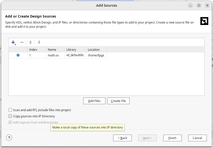
So let's add the original j_math module that did 3*x+10000 to our IP. In the IP project, go to add/create sources and in that window go to add source. Find the j_math.sv file. Be careful with the next step. Instead of leaving the box checked that says make a copy, instead uncheck that. What this will let you do is continue to edit that file outside of Vivado and it will just continually use your edited copy as you make changes (however maybe consider not having the Vivado edit window and VSCode open at the same time avoid collissions).

If you don't have a copy of j_math.sv from the previous pages, what is wrong with you? jk. here's a copy:

module j_math #
	(
		parameter integer C_S00_AXIS_TDATA_WIDTH	= 32,
		parameter integer C_M00_AXIS_TDATA_WIDTH	= 32
	)
	(
		// Ports of Axi Slave Bus Interface S00_AXIS
		input wire  s00_axis_aclk, s00_axis_aresetn,
		input wire  s00_axis_tlast, s00_axis_tvalid,
		input wire [C_S00_AXIS_TDATA_WIDTH-1 : 0] s00_axis_tdata,
		input wire [(C_S00_AXIS_TDATA_WIDTH/8)-1: 0] s00_axis_tstrb,
		output logic  s00_axis_tready,

		// Ports of Axi Master Bus Interface M00_AXIS
		input wire  m00_axis_aclk, m00_axis_aresetn,
		input wire  m00_axis_tready,
		output logic  m00_axis_tvalid, m00_axis_tlast,
		output logic [C_M00_AXIS_TDATA_WIDTH-1 : 0] m00_axis_tdata,
		output logic [(C_M00_AXIS_TDATA_WIDTH/8)-1: 0] m00_axis_tstrb
	);

  logic m00_axis_tvalid_reg, m00_axis_tlast_reg;
  logic [C_M00_AXIS_TDATA_WIDTH-1 : 0] m00_axis_tdata_reg;
  logic [(C_M00_AXIS_TDATA_WIDTH/8)-1: 0] m00_axis_tstrb_reg;

  assign m00_axis_tvalid = m00_axis_tvalid_reg;
  assign m00_axis_tlast = m00_axis_tlast_reg;
  assign m00_axis_tdata = m00_axis_tdata_reg;
  assign m00_axis_tstrb = m00_axis_tstrb_reg;
  assign s00_axis_tready = m00_axis_tready;

  always_ff @(posedge s00_axis_aclk)begin
    if (s00_axis_aresetn==0)begin
      m00_axis_tvalid_reg <= 0;
      m00_axis_tlast_reg <= 0;
      m00_axis_tdata_reg <= 0;
      m00_axis_tstrb_reg <= 0;
    end else begin
      if (m00_axis_tready)begin
        m00_axis_tvalid_reg <= s00_axis_tvalid;
        m00_axis_tlast_reg <= s00_axis_tlast;
        //m00_axis_tdata_reg <=3*s00_axis_tdata+10000;
        m00_axis_tdata_reg <=s00_axis_tdata;
        m00_axis_tstrb_reg <= s00_axis_tstrb;
      end
    end
  end
endmodule

What we'd like to do is drop that into our IP (and remove those two slave/master controller modules in the process. I dropped mine in like shown below (I saved you the time of manually typing out and matching the ports...but you can see it isn't too bad.) Later on we'll be able to just swap in fir15 when we're feeling good.

	module math_doer #
	(
		// Users to add parameters here

		// User parameters ends
		// Do not modify the parameters beyond this line


		// Parameters of Axi Slave Bus Interface S00_AXIS
		parameter integer C_S00_AXIS_TDATA_WIDTH	= 32,

		// Parameters of Axi Master Bus Interface M00_AXIS
		parameter integer C_M00_AXIS_TDATA_WIDTH	= 32,
		parameter integer C_M00_AXIS_START_COUNT	= 32
	)
	(
		// Users to add ports here

		// User ports ends
		// Do not modify the ports beyond this line


		// Ports of Axi Slave Bus Interface S00_AXIS
		input wire  s00_axis_aclk,
		input wire  s00_axis_aresetn,
		output wire  s00_axis_tready,
		input wire [C_S00_AXIS_TDATA_WIDTH-1 : 0] s00_axis_tdata,
		input wire [(C_S00_AXIS_TDATA_WIDTH/8)-1 : 0] s00_axis_tstrb,
		input wire  s00_axis_tlast,
		input wire  s00_axis_tvalid,

		// Ports of Axi Master Bus Interface M00_AXIS
		input wire  m00_axis_aclk,
		input wire  m00_axis_aresetn,
		output wire  m00_axis_tvalid,
		output wire [C_M00_AXIS_TDATA_WIDTH-1 : 0] m00_axis_tdata,
		output wire [(C_M00_AXIS_TDATA_WIDTH/8)-1 : 0] m00_axis_tstrb,
		output wire  m00_axis_tlast,
		input wire  m00_axis_tready
	);
  //throw out the caca that xilinx put here and replace with our module
  //there stuff is good, but we don't need it. We're making a simple
  //passthrough calculator-type device that handles AXIS spec on its own
  //either by being simple (the 3*x+10000 thing) or by designing it into
  //the the module (the FIR15 filter hopefully)

  j_math (  .s00_axis_aclk(s00_axis_aclk),
            .s00_axis_aresetn(s00_axis_aresetn),
            .s00_axis_tready(s00_axis_tready),
            .s00_axis_tdata(s00_axis_tdata),
            .s00_axis_tstrb(s00_axis_tstrb),
            .s00_axis_tlast(s00_axis_tlast),
            .s00_axis_tvalid(s00_axis_tvalid),

            .m00_axis_aclk(m00_axis_aclk),
            .m00_axis_aresetn(m00_axis_aresetn),
            .m00_axis_tready(m00_axis_tready),
            .m00_axis_tdata(m00_axis_tdata),
            .m00_axis_tstrb(m00_axis_tstrb),
            .m00_axis_tlast(m00_axis_tlast),
            .m00_axis_tvalid(m00_axis_tvalid)
        );
	endmodule

OK if this all went in, go through the re-packaging steps. There will likely be some "MERGE" things you need to click, but we're not dealing with any new ports or anything else weird, so this should just be easy to go and package. Finish and go back to your main project.

Back in Main Block Diagram

If you didn't already, add in your IP (and if you already did add it, make sure to upgrade the IP). We are now ready to wire it up. The only two things we want to manually route are the following:

• The Master AXIS port on the DMA to the Slave AXIS port on your math_doer IP.
• The Master AXIS port on the math_doer IP to the Slave AXIS port on the DMA.

We're essentially making a simple streaming loopback mechanism. Data will come from python/processor...get math "done" to it...then sent back into memory. Make sure you wire these correctly. Vivado sucks with its mouse handling.

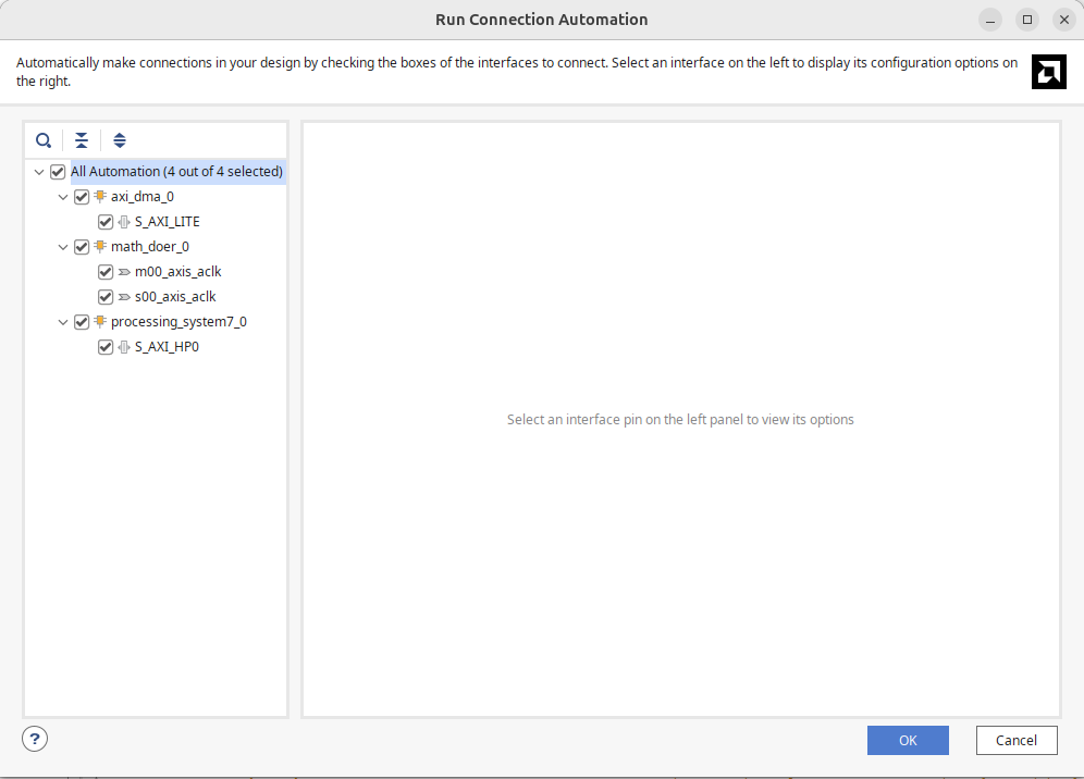
Once done, all the other wiring should be able to be automated. It will likely need to be done in two waves. The first time you do it you should have something like the following. Make sure all boxes are checked and let it run:

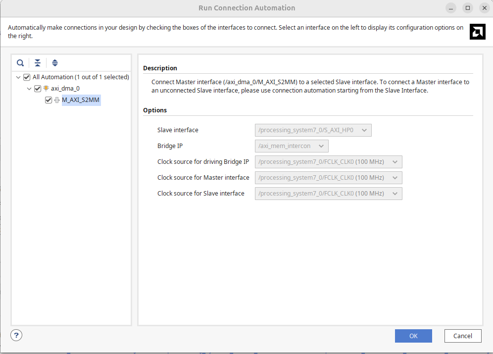
Then likely it'll prompt you a second time at the top. Run it again like the box below shows.

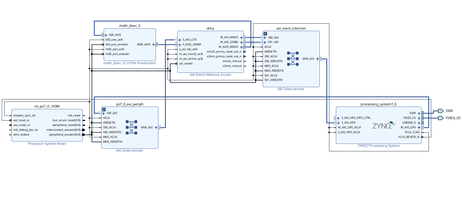
Once that is done you should have an overall design that looks like the following. The two Interconnects and the Processor System Reset are utility pieces of IP that should get automatically generated...only the Zynq Processor, the DMA, and the math_doer IP (or whatever you called yours) should be ones you actually added.

If this seems good, validate the design, Create the HDL wrapper, make sure it is the top level (it should be), and then do a build up through bitstream.

Into Python Land

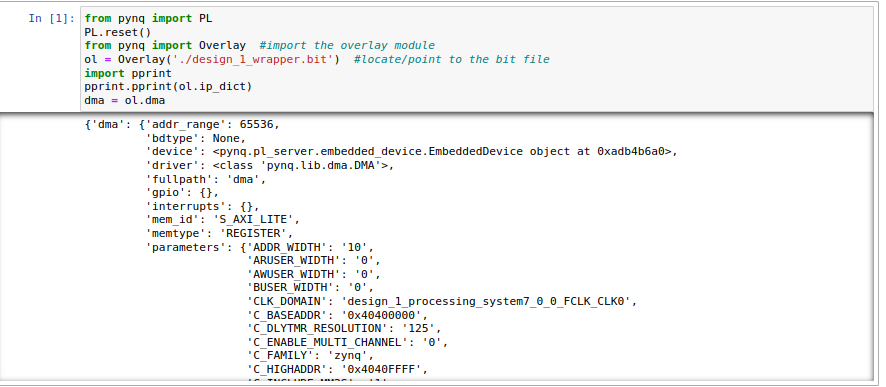
We now have a Python notebook we'd like to run. The first part is the following:

from pynq import PL
PL.reset() #important fixes caching issues which have popped up.
from pynq import Overlay  #import the overlay module
ol = Overlay('./design_1_wrapper.bit')  #locate/point to the bit file
import pprint
pprint.pprint(ol.ip_dict)
dma = ol.dma

The result of running this chunk should be this. If you do not see something basically very similar/identical, there is an issue with how something got generated.

The second part is a time-trial. It will run the identical data set on in software (using numpy or scipy functionality so it actually is fast and not artificially made to look bad with traditional Python bloat) and then compare it to your hardware accelerator. The data will get sent down over DMA interface and then put back into memory via the DMA interface. For this first "experiment" we're just comparing to our very simple j_math (3*x + 10000) math. 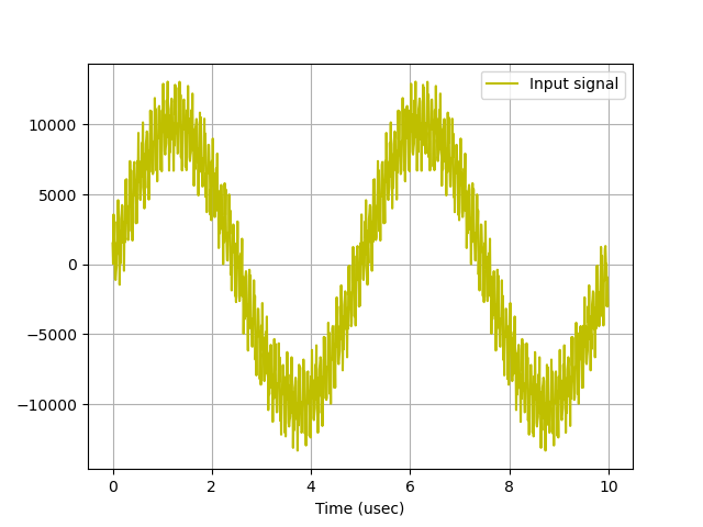So you'll see there's a line in python swresult = 3*samples+10000 doing that on the samples array which is 2 million elements long and contains a signal comprised of three sine waves of varying frequencies and amplitudes. That wave will look something like below (note yours might look a bit fuzzier since when I took this photo I had one of the high frequencies set at 12 MHz, but decided 20 MHz is better for this lab):

When this code is run, you should then get two identical plots:

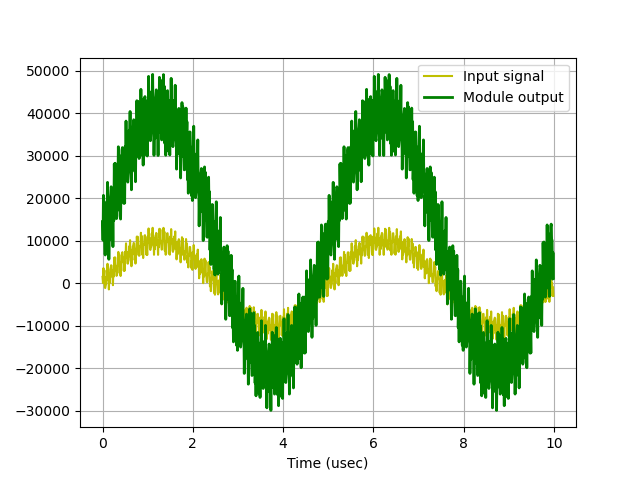
One of these plots is from the software calculation of scaling the signal by 3 and adding 10000 to it. The other is the result of the hardware doing it. Near each plot should be notifications of the time it took for software and hardware to do this. In running this you should see that the hardware is a bit faster than the software. In my repeated runs I was seeing factors of about four to five (in favor of hardware). You'll notice that the run-time for the hardware is going to be in the neighborhood of 20 to 30 milliseconds. This is largely based on the fact that the Streaming pipeline we have is running at 100 MHz and it is taking in 32 bits at a time. Since each value in our samples array is 4 bytes, we can handle one value every 10 ns and that means we need about ~20-ish milliseconds to calculate this data.

import numpy as np
from scipy.signal import lfilter
import time
%matplotlib notebook
import matplotlib.pyplot as plt
from scipy.signal import lfilter

def plot_to_notebook(time_sec,in_signal,n_samples,out_signal=None):
    plt.figure()
    plt.subplot(1, 1, 1)
    plt.xlabel('Time (usec)')
    plt.grid()
    plt.plot(time_sec[:n_samples]*1e6,in_signal[:n_samples],'y-',label='Input signal')
    if out_signal is not None:
        plt.plot(time_sec[:n_samples]*1e6,out_signal[:n_samples],'g-',linewidth=2,label='Module output')
    plt.legend()

# Total time of signal
#just create 20 ms of signal in python for testing and demo:
T = 0.02
# Sampling frequency
fs = 100e6
# Number of samples
n = int(T * fs)
# Time vector in seconds
t = np.linspace(0, T, n, endpoint=False)
# Samples of the signal
samples = 10000*np.sin(0.2e6*2*np.pi*t) + 1500*np.cos(46e6*2*np.pi*t) + 2000*np.sin(20e6*2*np.pi*t)
# Convert samples to 32-bit integers
samples = samples.astype(np.int32)
print('Number of samples: ',len(samples))

# Plot signal to the notebook
plot_to_notebook(t,samples,1000)


#my fir coefficients...maybe your's are different.
#change if different!
coeffs = np.array([-2,-3,-4,0,9,21,32,36,32,21,9,0,-4,-3,-2])
start_time = time.time() #just before operation run
#For first part just do the simple math operation we wanted:
#this is numpy array so it'll know how to do this operation
#in a pretty efficient manner!
swresult = 3*samples+10000

#lfilter is a decently fast way to run a fir in python
#there's some sites that compare, but it is in the running for
#among the good ones/most efficient.
#remember despite this being "python", it is really just Python
#calling highly optimized C operations (numpy and scipyi) written
# by better people than you or I, so this is a pretty decent
#test of a what a computer can do on the SW side.
#first arg is zeroes coefficients (which correspond to the
#delay taps of the FIR (the feed-forward coefficients)
#second arg is the feedback coefficients (poles coefficients)
#That'll be just 1 here since we're an FIR
#Third argument is the samples.
#uncomment for part 2 (And comment out the
#swresult = lfilter(coeffs, [1.0], samples)

stop_time = time.time() #just after operation run
sw_exec_time = stop_time - start_time
print('Software execution time: ',sw_exec_time)

# Plot the result to notebook
plot_to_notebook(t,samples,1000,out_signal=swresult)

#HARDWARE TIME
#now it is time to run on hardware:
from pynq import allocate
import numpy as np

# Allocate buffers for the input and output signals
in_buffer = allocate(shape=(n,), dtype=np.int32)
out_buffer = allocate(shape=(n,), dtype=np.int32)

# Copy the samples to the in_buffer
np.copyto(in_buffer,samples)

# Trigger the DMA transfer and wait for the result
start_time = time.time()
dma.sendchannel.transfer(in_buffer)
dma.recvchannel.transfer(out_buffer)
dma.sendchannel.wait()
dma.recvchannel.wait()
stop_time = time.time()
hw_exec_time = stop_time-start_time
print('Hardware execution time: ',hw_exec_time)
print('Hardware acceleration factor: ',sw_exec_time / hw_exec_time)
# Plot to the notebook
plot_to_notebook(t,samples,1000,out_signal=out_buffer)

# Free the buffers
in_buffer.close()
out_buffer.close()

Testing our FIR Filter

OK now here comes the big test. Somewhere on your computer place a copy of your quasi-verified fir15.sv module. Go back up your math_doer IP and let's add it into the IP. Take careful care TO NOT COPY IT IN!!!! REMEMBER THIS WILL LET YOU MODIFY IT/REPLACE EASILY OUTSIDE OF VIVADO!!!

Assuming you build the fir15 module using the provided axis skeleton, you should literally just be able to change the name of hte module instantiated in your IP top level to whatever your filter is called. Mine was called fir_15 so after a few keystrokes, I had:

  fir_15 (  .s00_axis_aclk(s00_axis_aclk),
            .s00_axis_aresetn(s00_axis_aresetn),
            .s00_axis_tready(s00_axis_tready),
            .s00_axis_tdata(s00_axis_tdata),
            .s00_axis_tstrb(s00_axis_tstrb),
            .s00_axis_tlast(s00_axis_tlast),
            .s00_axis_tvalid(s00_axis_tvalid),

            .m00_axis_aclk(m00_axis_aclk),
            .m00_axis_aresetn(m00_axis_aresetn),
            .m00_axis_tready(m00_axis_tready),
            .m00_axis_tdata(m00_axis_tdata),
            .m00_axis_tstrb(m00_axis_tstrb),
            .m00_axis_tlast(m00_axis_tlast),
            .m00_axis_tvalid(m00_axis_tvalid)
            );

Now, this should be all that's needed to change the IP (you can see the benefits of writing things to common busses with common naming schemes...it almost feels like it shouldn't be that easy.)

Rebuild your IP (approve all their merge notes or whatever). When done go back to your top level block diagram, regenerate all output products and rebuild the entire project. Your hardware handoff file should not need to be updated/replaced since from the outside everything about this design looks the same. The only stuff you've changed is what the streamin AXI module does.

When done, move that bit stream onto the Pynq file system, as one does, and let us return to the Python notebook. You'll need to re-run the reload part.

Let's go to the python file. Same as before...run that first part that loads the overlay (it is a new bit file with a juicy hopefully functioning FIR in it, after all). then before we go to the second part, let's update it a bit.

Previously we were doing a race of the math function f(x)=3x+10000. Now we're doing a 15-point convolution (FIR filter). We need to do an apples-to-apples comparison. Comment out the line:

swresult = 3*samples+10000

and now uncomment the line. This is one way to compute (quite quickly) the application of an FIR filter to a signal. This will be what we compare against.

swresult = lfilter(coeffs, [1.0], samples)

Note this is using a array defined above that I have filled with my fir coefficients. If your's are different, replace them!

coeffs = np.array([-2,-3,-4,0,9,21,32,36,32,21,9,0,-4,-3,-2])

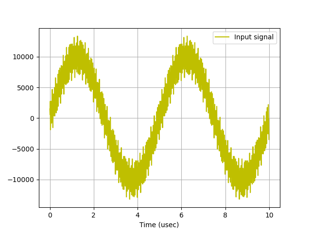
Once this is done, run it again. The starting signal should look like this again. It is comprised of three sine waves of various frequencies and amplitudes:

• A large amplitude sine wave at 200 kHz
• A small amplitude sine wave at 46 MHz
• Another small amplitude sine wave at 20 MHz

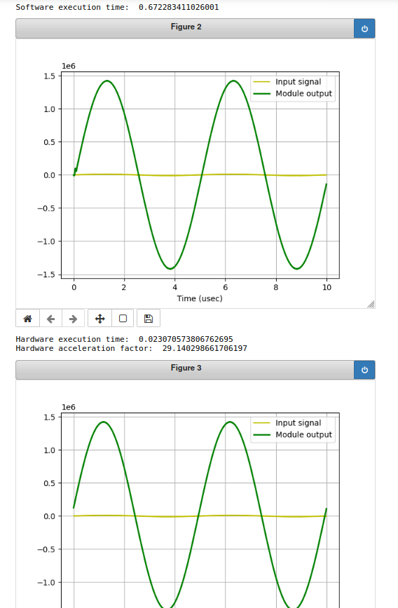
If we run the python script that does both the software FIR and hardware FIR we should get two (hopefully) identical-looking (hopefully) plots out. And the hardware acceleration factor should be on proud display here...I was getting a factor of ~30 in repeated runs here. That's pretty cool.

Remember, our filter is a low-pass, letting stuff below 10 MHz through and killing off above it. We should expect just the pure low-frequency sine wave to make it through and you should see that. You may also see that the resulting signal (in both case) has greatly amplified the sine wave...this is because our FIR filter coefficients are all integers (rather than floats that are normalized to 1). The general shape of our response is correct, it is just scaled due to fact that our coefficients are so large overall (though the same relative values to one another). If you wanted to get back to the original signal, you'd need to divide (or hopefully shift down) by the amount of the filter gain which is something in the neighborhood of 140 for this filter (you can roughly gauge this by summing all the FIR coefficient weights).

The reason the acceleration is better now than it was for the simpler math operation is because of how much "math" needs to be done...for the application of 3*x+10000, you just need to do one multiply-add per value...that's not too tough for a processor to do...but now we're doing on about fifteen multiply-adds per sample...the processor still has to effectively do those one at a time, whereas our FIR filter should be doing so with a pipeline, in effect spreading all that work out over a bunch of different stages all running at once. Math in pipelined hardware scales super easily...you might notice that the total time our hardware to calculate the FIR is still about 20 milliseconds or so. It is still doing its math about as fast as before (minus the ~150 ns of added latency which is hard to detect). By building up a pipelined FIR, we now have activated roughly fifteen times more compute than before, so we can still keep up. The processor is still stuck with its program counter and limited ability to do a fixed nubmer of instructions per cycle.

For larger and larger tasks (let's say a 1000 point FIR), the processor's performance will continue to get worse and worse in terms of time, where the FPGA will be able to keep up with the speed/throughput it has now if we just add more pipelined stages. Right now it is a factor of 30, but orders of magnitude higher are easy to imagine for larger tasks.

This is really starting to touch on the power of a hybrid environment like this. Nobody wants to write high-level commands in verilog. Python is good for that. But Python (and even Python calling gold-standard C operations like lfilter) just are not the best use of time of a processor if you can instead offload that to the customizable fabric. And that will only be beneficial if you can get your data in and out quickly (so not UART lol) and that's what DMA provides to us!

Nice.

Issues

If your system if freezing when running the code above there is likely an issue with either you dropping values or you dropping the TLAST signal. Return to your design and make sure that your verification code is

If your system is passing data, but the data looks like trash, that's actually less of a problem. (the TLAST/delay problems are trickier imo). first, check your sign math. Our FIR needs to be doing signed multiply adds...make sure you're obeying all rules when it comes to Verilog signed math!!!

When done, do some uploads...or show me in lab....or both...I don't need a video this week so the benefit of showing me live is reduced for sure.

Please upload a zip folder of your top level and inner-top-level .v file (the product of all the block diagramming),file.

Select File No file selected

Ask for Help Loading...

Please upload a couple screenshots in a zip of your accelerator running and depicting your hardware acceleration factor.

Select File No file selected

Ask for Help Loading...